Abstract
What should be measured when an artificial system begins to move from task performance toward strong intelligence? Current AI is usually evaluated externally, by benchmarks, outputs, and reward. Here we propose a different object of measurement: the internal regime organization created by learning. In prior work on Bernadotte Oscillatory Intrinsic Dimension (BOID), brain states were shown to be organized not by maximal complexity, but by regulated oscillator dimensionality: healthy brains expand dimensionality for conscious engagement and contract it for recovery, anaesthesia, sleep, or efficient trained control, whereas pathological states can reveal failure of dimensional regulation. This suggests a structural question for artificial intelligence: do trained neural networks also develop measurable internal regimes?
We investigate this question by analysing latent trajectories of trained networks with delay embeddings, Multichannel Singular Spectrum Analysis (MSSA), Koopman-mode analysis, BOID-style oscillatory dimensionality, regime-specific operators, and causal mode interventions. In a Continuous Thought Machine trained on maze solving, learning moves input-excited modes toward the unit circle, creates functional rhythms above the aperiodic background, and separates computation into a high-dimensional desynchronised working regime and a low-dimensional synchronised resting regime. Beyond the training horizon, the system alternates between work and rest, replays its solution, stores the answer in accumulated synchronisation, and restarts through a clock-like mode in the one-step dynamics.
These regimes are functional, not metaphorical. Removing specific rotating mode pairs selectively disrupts route content or abolishes the restart clock, while removing random planes has little effect. A reduced construction based on rotations plus a small learned correction partially rebuilds the trained dynamics with far fewer parameters. At the same time, the result is architecture-dependent: some trained systems acquire oscillatory regimes, stores, clocks, and replay, whereas others remain relaxation-like, line-like, or input-driven.
We therefore propose regime switching as a measurable structural marker for studying the transition from task-performing artificial systems toward strong artificial intelligence. The result is not that neural networks are brains, nor that larger models are necessarily more intelligent. The result is that learning can create functional internal dynamics, and that this dynamics can be measured. This work defines a programme for analysing intelligence through intrinsic dimensionality, topology, oscillator structure, regime autonomy, and the geometry of possible behaviour spaces.
Keywords: Continuous Thought Machines; MSSA; Koopman modes; Oscillatory dimensionality; Dynamical systems; Neural networks; Interpretability; Strong Artificial Intelligence; BOID
1. Introduction
Artificial intelligence is usually evaluated from the outside. A system is judged by the tasks it solves, the benchmarks it passes, the text it produces, the actions it selects, or the reward it maximizes. This external view has been extraordinarily productive, but it leaves open a deeper question: what kind of internal organization must a system acquire in order to move from task performance toward strong intelligence? The premise of this paper is that the transition toward strong artificial intelligence is not primarily a question of scale, but a question of regime organization. A system becomes structurally interesting when it acquires internal states that can expand, contract, synchronize, desynchronize, store, replay, and switch in a functionally meaningful way.
The central proposal of this paper is that regime switching can serve as a measurable structural marker of the transition from task-performing artificial systems toward strong artificial intelligence. A system that only maps inputs to outputs remains externally defined, even if it performs well. A system that develops internal work and rest states, replay, stores, clocks, and mode-specific causal structure begins to acquire an internal dynamical organization that can be measured independently of its task score. In this sense, regime switching is not an implementation detail of a particular architecture, but a candidate criterion for identifying when learning has created functional internal dynamics.
The conceptual chain of the paper is:
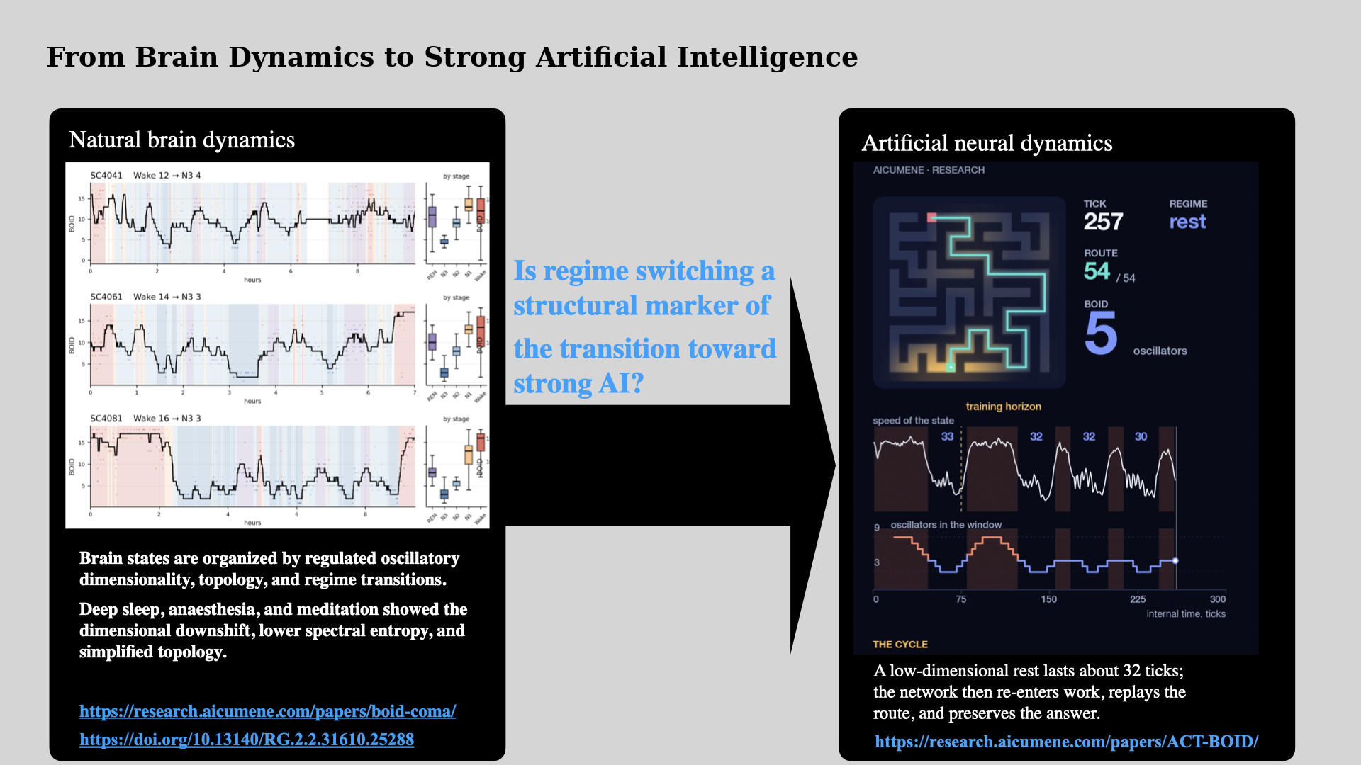
natural brain dynamics AI dynamics regime switching as a marker of the transition toward strong AI.
In previous work on Bernadotte Oscillatory Intrinsic Dimension (BOID), we showed that brain states are organized by regulated oscillator dimensionality: wakefulness, sleep, anaesthesia, meditation, recovery, and coma differ not simply by activity level or spectral power, but by intrinsic oscillatory dimensionality, topology, and regime transitions [1]. Here we ask the corresponding question for artificial neural systems: if natural intelligence is organized by measurable regimes, do trained neural networks also develop such regimes during learning?
The breakthrough claim is not that artificial neural networks are biological brains. The claim is sharper: brain dynamics reveal a measurable principle of regime organization, and some trained artificial systems acquire analogous regime structure. Others do not. This difference between architectures is not a limitation of the analysis, but the central result. It suggests that regime switching, intrinsic dimensionality, topology, stores, clocks, and replay may serve as structural markers for distinguishing task-performing systems from systems that begin to approach strong artificial intelligence.
This paper builds on a sequence of works in which oscillatory source estimation, topology-driven classification, BOID-style brain-state analysis [2, 1, 3, 4, 5, 6], trusted artificial intelligence and automata-based structural safety [7, 8, 9], semantic trajectories [10, 11, 12, 13], small neural architectures [14, 15], and structural criteria for strong intelligence [16] were developed as parts of a common programme. The common premise of this programme is that intelligence, trustworthiness, and cognitive organization should not be characterized only by outputs, but also by the geometry, topology, intrinsic dimensionality, and dynamics of the trajectories generated by the system.
Natural intelligence suggests why this shift is necessary. The brain is not a static input–output device. It is a dynamical system that moves between distinct internal regimes: wakefulness, sleep, anaesthesia, coma, recovery, focused work, rest, replay, and pathological suppression [1, 17, 18, 19, 20, 21, 22, 23, 24, 25]. These states are not distinguished only by behavioural labels or by changes in spectral power. They differ in the geometry of their trajectories, in the topology of their state-space organization, and in the effective number of oscillatory modes that remain active [1, 3, 19, 21, 23]. In the BOID framework, these differences are treated as measurable structural properties of brain-state dynamics [1, 3].
The central idea of BOID is that healthy brain function is not maximal complexity. It is regulated dimensional switching. A healthy brain must expand its active dynamical repertoire during conscious engagement, cognition, perception, action, memory, and internal simulation; but it must also contract this repertoire during sleep, anaesthesia, recovery, and trained efficient control [1, 3]. In this view, consciousness is not simply high activity, recovery is not simply low activity, and coma is not simply unconsciousness. They are different regimes of dimensional control. High dimensionality can be adaptive in the intact engaged brain, low dimensionality can be adaptive in recovery or trained control, and high dimensionality can become pathological after injury when it reflects fragmented mode proliferation rather than functional richness [1, 3].
This distinction is crucial. Deep sleep and propofol anaesthesia are not merely states of reduced signal amplitude; they are organized low-dimensional regimes in which the active oscillator repertoire contracts. In the BOID study, propofol sedation reduced BOID within subjects even in the presence of organized alpha activity, showing that BOID is not a band-power measure but a measure of the number of dynamically independent oscillatory modes required to generate the signal [1]. Expert meditation provided a complementary waking case: reduced intrinsic dimensionality can occur without loss of function, indicating an efficient control regime rather than collapse. Coma, by contrast, exposed the pathological boundary condition: in poor-prognosis post-anoxic coma, high BOID can mark disorganized mode proliferation and failure to downshift into a coherent low-dimensional recovery state [1, 3]. Thus, the biological variable of interest is not complexity itself, but the regulation of complexity across state transitions.
The methodological point is equally important. BOID is not a metaphorical description of brain complexity. It is obtained by reconstructing multichannel brain activity as a delay-coordinate trajectory and estimating the active oscillatory degrees of freedom within that trajectory. Multichannel Singular Spectrum Analysis (MSSA), developed by Bernadotte and Menshikov, provides the core instrument for this reconstruction [2]. A multichannel recording is embedded as a block-Hankel trajectory; the resulting trajectory space is decomposed into oscillatory components, low-dimensional trends, and background activity; and pole-estimation procedures such as ESPRIT recover the active damped exposinusoidal modes [2, 26, 27, 28, 29]. MSSA therefore does not merely filter a signal. It exposes the latent oscillator architecture through which a dynamical system expresses its state. The count and organization of these modes make regime structure visible.
This is the point at which the brain programme becomes relevant for artificial intelligence. If natural intelligence is organized by regulated dynamical regimes, and if these regimes can be measured through oscillatory dimensionality, topology, and trajectory geometry, then the internal dynamics of trained artificial systems becomes a central object of study. The question is not whether artificial networks are biological brains, nor whether all trained networks become brain-like. The question is more selective and more structural: do some trained artificial systems acquire internal dynamical regimes that are comparable, at the level of organization, to regime structure in natural intelligence? Do they develop high-dimensional working states, lower-dimensional resting states, functional modes, stores, clocks, and replay? Are these objects merely descriptive, or are they predictive and causally necessary for computation?
This question connects directly to structural criteria for strong artificial intelligence. In the Bernadotte–Gromov framework, strong intelligence is not defined by human imitation or by benchmark performance alone, but by internal criteria: intrinsic dimensionality, topological organization, dynamical autonomy, self-stabilizing regimes, and the capacity to reorganize internal state space in a functionally meaningful way [16]. Thus, the strength of an intelligent system is linked not only to the quality of its answers, but to the structure of the space of possible behaviours it can generate, stabilize, and transform. On this view, intelligence is not exhausted by input–output competence. A system approaches strong intelligence only when it acquires an internal state-space organization capable of sustaining, switching, compressing, expanding, and reusing its own dynamical regimes. Such a system must not only answer, classify, or act; it must maintain an organized internal world of trajectories, constraints, modes, and transitions.
Related work on trusted generative AI, probabilistic truth, and automata-based structural safety extends this structural view to agentic systems. There, safety is treated not only as output filtering, but as dynamic structural safety: an AI agent should be monitored through intrinsic dimensionality, topology, dynamical complexity, structural novelty, and BOID-like regime indicators [9, 7, 8]. This matters because a system may remain superficially compliant at the level of individual outputs while moving into a new, unvalidated behavioural regime. Trustworthiness and strength of an intelligent system are therefore both connected to the organization of its possible behaviour space, not merely to the apparent correctness of isolated responses. In parallel, the Spot the Bot programme studies human and machine-generated texts through semantic trajectories, clustering, information-theoretic structure, and intrinsic geometry of language space [10, 11, 12, 13]. Together, these works motivate a common principle: intelligent and trustworthy systems should be evaluated not only by their outputs, but by the geometry, topology, dimensionality, and dynamical regimes of the trajectories they generate.
This structural view is also consistent with our earlier work on small, lightweight, and locally deployable neural systems. In BCI and EEG applications, Hankel embeddings and compact pipelines were used to estimate the number of signal sources and to perform real-time EEG filtering and classification without relying on large end-to-end architectures [5, 4]. Counter-augmented deterministic automata provide a complementary example: a compact structural modification of the automaton avoids state explosion in real-time regular-expression matching while preserving deterministic behaviour [8]. In medical imaging and robotic neurosurgery, the Scientific Data brain-vessel dataset and VeNet show how carefully structured, resource-efficient pipelines can support segmentation, reconstruction, and endovascular robotic workflows under limited-data and resource-constrained conditions [15, 14]. The broader LevshaAI line connected such perception modules to patient-specific vascular simulation, haptic feedback, and intelligent robotic endovascular workflows [30, 31, 32].
This is important because the present paper does not claim that a larger model became intelligent. It argues almost the opposite: learning can create functional internal dynamics. The relevant object is not parameter count alone, but the emergence of organized modes, functional decomposition, internal clocks, stores, replay, and regime switching. Small, compact, and lightweight networks are therefore not peripheral to the argument. They support the central thesis: structurally interesting dynamics can emerge without scaling a model into a giant LLM. Compact systems can become structurally powerful when analytical operators, embodied constraints, functional decomposition, and regime dynamics are built into the architecture.
We therefore treat trained neural networks as learned dynamical systems. Rather than asking only whether a model solves a task, we ask what dynamical structure learning has created inside it. We analyse latent trajectories with delay embeddings, MSSA, Koopman-mode analysis, BOID-style oscillatory dimensionality, linear and regime-specific operators, and direct interventions on learned modes [2, 33, 34, 35, 36, 37, 38, 39]. This approach allows us to compare artificial systems not only by accuracy, but by their internal dynamical organization: whether they form oscillatory regimes, whether those regimes switch, whether modes are synchronized or desynchronized, whether a low-dimensional rest state exists, and whether the resulting structure is functional.
The central empirical case is a Continuous Thought Machine trained on maze solving [33]. We show that learning moves input-excited modes onto or near the unit circle and produces a small set of rhythms above the aperiodic background. Computation separates into a high-dimensional desynchronised working regime and a low-dimensional synchronised resting regime. A shared delay-coordinate operator predicts most of the step-to-step state change, while regime-specific operators describe work and rest but fail across regimes. When the network is left running beyond its training horizon, it alternates between work and rest, replays its solution, stores the answer in accumulated synchronisation, and restarts through a clock-like mode visible in the spectrum of the one-step map.
These dynamical objects are not only descriptive. Removing individual rotating mode pairs from the running network selectively disrupts route content or abolishes the restart clock, whereas removing random planes of the same dimension has little effect. Conversely, the same objects are partially constructive: replacing the recurrent core with a bank of rotations plus a small learned correction approaches the full model with substantially fewer parameters. Modes, regimes, stores, clocks, and replay are therefore not post hoc metaphors. They are measurable, predictive, causally testable, and partially buildable components of the learned system.
The broader result is architectural diversity. Across trained systems, the same measurements separate networks into oscillators with regimes, relaxations, lines, and driven streams. Some architectures acquire clear work–rest switching, endogenous clocks, replay, and functional oscillatory modes. Others do not. This diversity is not a weakness of the result; it is the result. It shows that regime organization is not an automatic consequence of training or scale. It is an emergent structural property of particular learning systems. That property can be measured, compared, perturbed, and potentially engineered.
Thus, this paper should not be read as another analysis of Continuous Thought Machines. It proposes a broader programme: a new programme for measuring the internal dynamics of intelligence. CTM is the first artificial test object in this programme because it provides a trained neural system in which work–rest switching, oscillatory modes, clocks, stores, replay, and causal mode interventions can be observed directly. The broader aim is to develop a structural science of intelligence in which natural brains and artificial systems can be compared through measurable properties of their internal dynamics rather than through behavioural analogy alone.
The contribution of this work is therefore threefold. First, we extend the BOID and MSSA programme from natural neural systems to artificial neural systems [1, 2, 3]. Second, we show that some trained networks develop functional dynamical regimes: working states, resting states, replay, stores, clocks, and mode-specific causal structure, while other architectures remain dynamically different. Third, we connect these findings to structural criteria for strong artificial intelligence, trusted AI, and small-AI architectures, where internal dimensionality, topology, structural novelty, regime transitions, operator-aware design, compact structural automata, and functional decomposition are treated as measurable properties of intelligent systems rather than metaphors [16, 9, 14, 15, 30, 8, 10, 13].
We propose that regime switching is one of the first measurable structural markers by which the transition from task-performing artificial systems toward strong artificial intelligence can be studied experimentally.
Figure 1 summarizes the conceptual chain of the paper: natural brain dynamics motivate BOID, BOID becomes measurable through MSSA, MSSA and Koopman analysis define the artificial-network measurement language, and trained networks provide the test bed for regime switching as a structural marker of strong artificial intelligence.
1.1 The technical question and the outline of the argument
Having stated the structural hypothesis, we now formulate the technical question. Any system that learns to compute by iterating – a recurrent network over a sequence, a reasoning network over its own internal steps, a language model over generated text, or a cortex over time – does its work through the evolution of a state. Training fixes the weights; what it shapes is a dynamics. The question is therefore not only what the system outputs, but what internal dynamical structure learning has created: which modes are sustained, which regimes are entered, which operators govern them, and which components are causally necessary for computation.
The article is organized as follows. Section 2 gives a unified spectral-dynamical framework: Hankel trajectories, MSSA, Bernadotte oscillator expansion, BOID-style oscillatory dimensionality, Koopman modes, regime-specific operators, and hybrid spectral architectures. Section 3 fixes the model system and measurement protocol. Section 4 reports the first group of results on the maze CTM: learning-created sustained modes, training dynamics, and dimension as computation in progress. Section 5 analyses the operator structure, work–rest–replay cycles, holding, restarting, causal mode ablations, and clock-like modes. Section 6 asks what sets the regime pattern by varying memory length, comparing an LSTM control, and constructing hybrid spectral cores. Section 7 compares other learning systems measured with the same signature. Section 8 relates the dynamical invariants to cognitive functions. Sections 9 and 10 state the scope of the results and conclude.
2. A unified spectral-dynamical framework
The purpose of this section is to make explicit the bridge from BOID and MSSA to trained artificial neural systems. The framework has four steps. First, a multichannel trajectory is embedded into a Hankel trajectory space. Second, MSSA decomposes this trajectory into oscillatory subspaces, low-dimensional trends, and background activity. Third, the active oscillatory modes define a BOID-style intrinsic oscillatory dimensionality. Fourth, for trained neural networks, these modes are interpreted as Koopman modes of the iterated map generated by the network. This makes it possible to compare biological brain states and artificial latent trajectories in the same structural language: modes, dimensions, operators, regimes, stores, clocks, and switches.
The framework is not intended to claim biological identity between brains and artificial networks. Its aim is structural. A biological brain state and an artificial latent state may be generated by different mechanisms, but both can be treated as trajectories of a dynamical system. If those trajectories can be embedded, decomposed, counted, and perturbed in the same mathematical language, then one can ask whether the same types of dynamical organization occur in both domains. This is the role of MSSA and BOID in the present work: they provide a measurement language for internal regime organization.
2.1 From brain regimes to learned neural regimes
The BOID programme begins from the observation that brain states are not arranged on a single monotonic axis from low to high complexity. Wakefulness, sleep, anaesthesia, meditation, recovery, and coma differ by the regulation of active oscillatory degrees of freedom. In healthy states, the brain can expand its active repertoire during conscious engagement and contract it during sleep, anaesthesia, recovery, or efficient trained control. In pathological states, high apparent dimensionality may instead reflect fragmented mode proliferation and failure to downshift into a coherent recovery regime [1].
This suggests a structural hypothesis for artificial intelligence. If natural intelligence is organized by regulated regime switching, then trained artificial systems should not be evaluated only by their outputs. Their internal trajectories should also be examined for the emergence of regimes: high-dimensional working states, low-dimensional resting states, replay, stores, clocks, synchronization, desynchronization, and mode-specific causal structure. The central question is therefore not whether artificial networks are brains, but whether learning can create measurable internal regime organization in artificial systems.
2.2 Hankel trajectories and MSSA
Let be a multichannel record. Equation (1) defines the observable multichannel trajectory used throughout the paper. The channels may be EEG derivations, pooled neuronal populations, hidden units of a recurrent network, latent coordinates of an artificial system, or any other set of observables sampled along an internal or external time index. Given an embedding length , the Hankel trajectory matrix is constructed by stacking consecutive samples: Equation (2) is the trajectory object on which MSSA, BOID-style dimension, and operator fitting are built. For a multichannel signal, each is itself a vector, so is a block-Hankel matrix. This embedding transforms temporal evolution into a geometric trajectory in a higher-dimensional space. Under standard delay-coordinate assumptions, such an embedding reconstructs the state-space structure of the underlying dynamical system up to a change of coordinates [28, 29, 40].
MSSA applies singular value decomposition to the trajectory matrix: The decomposition in Equation (3) gives the leading singular subspaces that describe the dominant geometry of the trajectory. Oscillatory components appear as approximately paired singular directions corresponding to rotating structures in the embedded space. Low-dimensional trends, transient components, and background activity occupy different parts of the singular spectrum. Thus MSSA does not merely smooth or filter a signal. It converts a temporal record into an explicit geometric object whose modes, dimensions, and oscillatory structure can be measured [2, 27, 41].
2.3 Bernadotte oscillator expansion
The Bernadotte oscillator expansion represents a multichannel trajectory as a superposition of exponentially modulated oscillatory components: Equation (4) is the explicit spectral form used to interpret damped, sustained, and growing modes. Each component is defined by an amplitude , a growth or decay coefficient , a frequency , and a phase . This generalizes ordinary Fourier decomposition by allowing damping, transient growth, metastability, and nonstationary oscillatory behaviour. A mode with is damped, a mode with is sustained, and a mode with grows until bounded by nonlinear effects.
This representation is well suited to brain and neural-system dynamics because such systems are rarely stationary sums of pure sinusoids. They switch regimes, damp and revive modes, synchronize and desynchronize populations, and produce transient trajectories. The relevant object is therefore not simply spectral power in a fixed frequency band, but the active oscillator architecture that generates the observed trajectory.
2.4 BOID-style oscillatory dimensionality
We define the intrinsic oscillatory dimensionality of a state or trajectory as the effective number of active oscillatory modes required to generate it: Equation (5) is the BOID-style quantity that is compared across brain states and artificial regimes. In the brain-state setting, this is the Bernadotte Oscillatory Intrinsic Dimension (BOID). In the artificial-network setting, we use the same principle in a BOID-style sense: counts the active oscillatory degrees of freedom excited by the network, the task, or the regime under measurement.
Operationally, can be estimated in several complementary ways. The first is the signal-subspace rank of the Hankel trajectory matrix, with appropriate energy or surrogate thresholds. The second is pole estimation, for example by ESPRIT, which recovers damped exposinusoidal modes from the delay-coordinate subspace [26]. The third is a Monte-Carlo SSA or aperiodic-background control, which counts oscillatory components that rise above coloured -like background activity [41].
This distinction matters. A broadband participation ratio may measure how much of the trajectory space is being used, while a surrogate-thresholded oscillator count measures how many rhythms stand above the aperiodic background. These quantities need not coincide. In biological brain recordings, dimensionality and synchrony can dissociate. In the maze CTM analysed below, dimension and synchrony move together across work and rest. The framework therefore does not assume a single scalar complexity measure. It separates oscillatory count, broadband dimension, synchrony, damping, and regime structure.
2.5 Trained networks as iterated maps
A trained neural network can be treated as a dynamical system whenever it repeatedly updates an internal state along some index. The index may be the internal tick of a CTM, the position in a sequence, the step of an iterative reasoner, the denoising step of a diffusion sampler, the generated-token axis of a language model, or the time index of a biological recording. In the general discrete-time case, the network acts on a state by where is the input or drive present at step .
When the input is held fixed, removed, or explicitly regressed out, the autonomous part of the dynamics can be written as Equations (6) and (7) distinguish driven trajectories from the internal map whose modes we estimate. This is the setting in which the internal dynamics of the trained system can be studied most directly. The question is then not only what output the network produces, but what map training has created: whether the state contracts to a fixed point, follows a line, remains driven by external input, or develops sustained oscillatory regimes with work–rest switching, clocks, stores, and replay.
This discrete formulation is the primary one used in the present paper. Continuous-time notation may be useful as an approximation, but the empirical measurements below use sampled trajectories rather than Equation (8) directly; they are made on sampled trajectories and iterated maps. The relevant object is therefore the one-step or finite-step evolution of the learned state.
2.6 Koopman modes of trained networks
For an autonomous iterated map , the Koopman operator acts linearly on observables of the state: Although the state map may be nonlinear, the Koopman operator is linear on the space of observables. If is a Koopman eigenfunction, then along a trajectory Equations (9)–(11) explain why oscillatory modes can be read as modes of the learned map. For real-valued dynamics, complex eigenvalues occur in conjugate pairs. Writing one obtains the same exposinusoidal component that appears in the Bernadotte oscillator expansion: Equation (12) therefore connects Koopman spectra to the oscillator expansion of Equation (4). Thus the oscillatory modes extracted from delay-coordinate trajectories can be interpreted as Koopman modes of the trained network’s iterated map [35, 36, 37, 38, 39, 34].
This observation is the mathematical bridge between MSSA, BOID, and neural-network dynamics. In brain recordings, the modes describe active oscillatory degrees of freedom of the biological system. In trained networks, they describe the oscillatory degrees of freedom of the learned map, or of the part of the map that is visible in the chosen observables. A mode on or near the unit circle is sustained. A mode inside the unit circle is damped. A mode outside the unit circle grows until constrained by nonlinear saturation or regime switching.
2.7 Regime-specific operators
In a system with distinct regimes, a single global operator may describe part of the dynamics, but different regimes may require different local operators. We therefore distinguish between a shared operator , fitted across all trajectories and all regimes, and regime-specific operators such as and . If predicts work but fails on rest, and predicts rest but fails on work, then the system is not merely moving along one homogeneous trajectory. It is switching between distinct dynamical regimes.
This distinction is central for the present paper. In the maze CTM, the dynamics is approximately linear within a regime, while the nonlinearity is concentrated in the switch between regimes. A work operator describes the high-dimensional desynchronised computational phase. A rest operator describes the low-dimensional synchronised phase. Neither operator transfers well to the other regime. The switch itself is therefore a structural event, not just a change in speed or amplitude.
2.8 Hybrid spectral architectures
The same framework also suggests a constructive architecture. Instead of treating a trained recurrent core as a black box, one can decompose it into an explicit spectral operator plus a learned correction: Here is the linear spectral component estimated from MSSA, delay-coordinate DMD, or the Koopman restriction to the observed trajectory subspace, while represents the residual nonlinear correction. In continuous notation the same idea is written as The discrete form in Equation (13), rather than Equation (14), is the one used for the empirical networks in this paper.
In a regime-structured system, the decomposition may become Equation (15) is the operator form of regime switching used in the interpretation of work and rest. The operator captures the local oscillatory geometry of regime , while the learned correction and the switching mechanism account for transitions between regimes. If the residual is small within regimes and large at switches, then the architecture is interpretable as a set of spectral cores connected by learned transitions.
This gives a constructive interpretation of the measurements. Modes are not only descriptive summaries of trajectories. They can be written into the architecture as rotation banks, damped oscillators, or structured spectral operators. The experiments below test this idea by replacing a recurrent core with a bank of rotations plus a small learned correction. The result is not meant to show that all intelligence is oscillation, but that part of a trained computation can be carried by explicit oscillatory structure.
2.9 Regime organization and strong artificial intelligence
The framework becomes relevant to strong artificial intelligence because it gives operational meaning to internal structural organization. A system that maps inputs to outputs may be powerful, but it remains externally defined if its internal dynamics has no measurable regime structure. A system that develops internal modes, clocks, stores, replay, and regime-specific operators begins to acquire an organization that can be measured independently of task score.
In this sense, regime switching is a candidate structural marker of the transition from task-performing artificial systems toward strong artificial intelligence. The claim is not that the presence of oscillations is sufficient for strong intelligence. It is not. A network may oscillate without solving a task, and a system may solve a task through contraction, relaxation, or a driven stream. The claim is sharper: when learning creates functional regimes that can be measured, predicted, perturbed, and partially reconstructed, it creates internal dynamics of a kind that external performance metrics alone do not capture.
This is why architectural diversity is part of the framework rather than an exception to it. Some systems may be oscillators with regimes. Others may be relaxations to fixed points, lines, or driven streams. Comparing these dynamical classes is precisely how one asks whether a trained system has acquired regime autonomy, internal dimensionality, topology, and reusable state-space organization.
2.10 Scope of the framework
The framework applies whenever three conditions are met. First, the system must provide an index along which a state evolves. Second, it must provide channels whose values along that index can be treated as a multichannel record. Third, there must be a way to separate, at least approximately, the system’s autonomous dynamics from external drive.
These conditions are satisfied most directly by CTMs, where the input can be fixed and the internal tick axis exposes the evolution of the state. They are also partially satisfied by recurrent networks, state-space models, iterative inference systems, language-model generation, diffusion samplers, residual networks along depth, optimization trajectories, and biological recordings. The quality of the measurement depends on how well the autonomous dynamics can be separated from the drive. For this reason, the same instrument may reveal an oscillator with regimes in one architecture, a relaxation in another, a line in a diffusion sampler, or a driven stream in language generation or cortex.
Thus the framework is not a claim that all trained networks share the same dynamics. It is a measurement programme for determining what kind of dynamics learning has produced. The results below apply this programme first to a CTM trained on mazes, and then to a broader set of trained systems measured with the same signature.
3. The model system and the measurement protocol
This section turns (Section 2.4) into a measurement protocol [2, 1] for the released Sakana architecture [33]. It was written before any computation; the results are in Section 4.
3.1 What a CTM exposes
A Continuous Thought Machine [33] unfolds computation along an internal time axis of “ticks” that is decoupled from the input. Each of its neurons owns a small neuron-level model that maps a short history of its pre-activations (memory length ) to a post-activation (), = 1, ..., ; the representation that drives attention and the output is the pairwise synchronisation matrix () -() (), subsampled to a few hundred neuron pairs. The released code (Apache-2.0, with checkpoints for ImageNet, 2-D mazes, sorting, parity and question answering) can return the full post-activation history for every input, together with the per-tick predictions and certainties. In the terms of Section 2, is the multichannel signal () with = neurons as channels and the tick index as time.
3.2 Estimators
In Section 2.4, is the dimension of the subspace that a superposition of exposinusoidal modes occupies in Hankel embedding space. That this subspace is an invariant of the generating dynamics, with a dimension fixed by the number and type of the modes, is the result on which the definition rests [3]. The same work builds a classifier on the distance between such subspaces, which is a natural further read-out for CTM trajectories.
Three estimators of are available and already validated on EEG and on two-photon calcium imaging [1]: Oscillator count (BOID), Surrogate-thresholded dimension , and Aperiodic Monte-Carlo SSA index.
Oscillator count (BOID). Block-Hankel embedding of with lag , singular-value decomposition, signal-subspace rank by a 95 % energy criterion, TLS-ESPRIT poles [26], count of poles with positive frequency in a band of interest. Gives frequencies and dampings of the modes (the , of Section 2.3).
Surrogate-thresholded dimension . Size of the leading block of Hankel singular values that exceeds a null built from independent per-neuron temporal shuffles of the same window.
Aperiodic Monte-Carlo SSA index. Surrogates with the window’s own 1/ background projected on the observed eigendirections [41], with jPCA plane pairing; counts oscillators above the aperiodic background and yields their frequencies. This is the estimator to trust when the background is coloured, which is the typical case for learned dynamics.
Two properties of CTM data dictate the implementation. First, (hundreds to thousands of neurons, tens to a hundred-odd ticks): the trajectory matrix has rank at most = - + 1, and its spectrum is obtained exactly from the Gram matrix, which makes surrogate ensembles cheap even at = 2 048. Second, single neurons are the wrong channels for a dimension estimate, exactly as single cells were in calcium imaging: the count should be computed on a montage of pooled neuron groups (random tiles, or groups defined by the synchronisation pairs the model itself selects), with the granularity varied as a control.
3.3 Experimental design
Per-input dimensionality. For each input, of over the whole tick range, against the model’s own certainty and the tick at which it commits. Hypothesis: harder inputs (longer mazes, am- biguous images) sustain more modes for longer.
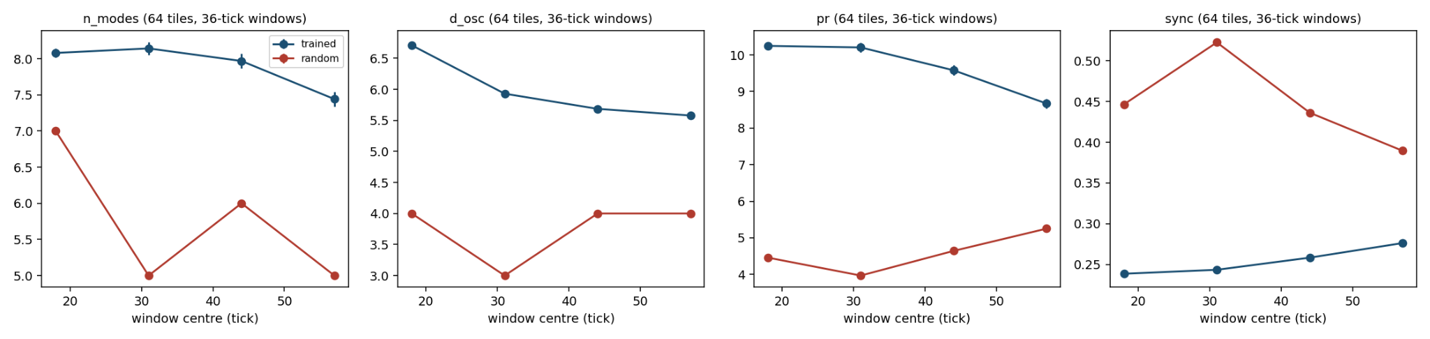
Along internal time. Sliding windows over ticks: does the mode count collapse as the model converges to a decision (damped modes, < 0), or does a persistent oscillatory repertoire remain?
Across training. The same measurement on checkpoints from initialisation to convergence: does training create oscillatory modes, prune them, or reorganise them into fewer, stronger ones? This is the direct test of the claim of Section 2.5 that CTMs learn oscillatory manifolds.
Against baselines. The repository ships non-temporal and LSTM baselines; their internal states give the null expectation for “modes” in a learned representation that has no synchronisation objective.
Count versus synchronisation. The CTM’s representation is pairwise synchronisation; is a mode count. On calcium data the two dissociated (dimension fell where synchrony did not, and vice versa); the same dissociation in a CTM would show that the model’s oscillatory repertoire is not reducible to the pairwise statistic it is trained on.
3.4 Pitfalls specific to CTMs
Short windows. With 50–150 ticks, must stay below /3, which limits the slowest resolvable mode to a few ticks per cycle; the count ceiling (-1)eff/2 must be reported with every number.
Non-stationarity. The tick axis is a transient, not a stationary record: the exposinus model handles damping explicitly, but shuffle nulls assume exchangeable samples, so the aperiodic null (estimator 3) should be the primary one and the white null a control.
Regime check. When the Hankel spectrum is nearly flat (participation ratio comparable to ), the leading-block count becomes unstable; the participation ratio is to be recorded alongside every count, as in the calcium study.
Emergent, not built-in, oscillation. Nothing in the architecture forces oscillation; the neuron-level models are small MLPs over a history. A high would therefore be a finding about what training produces, not a restatement of the architecture.
3.5 Cost and outcome
A first pass on the maze checkpoint — post-activation extraction with tracking enabled, the three estimators on a montage of 64 groups and on the raw neurons, the five contrasts above — is a few hours of work on a single RTX 4090, with the analysis code reused from the calcium study [1].
Its outcome is a figure set analogous to that study — by task difficulty, by internal time, by checkpoint, and the count against synchronisation — and, if the result is positive, the analytic operator of the hybrid architecture of Section 2.8, = +(), taken directly from the fitted modes. Section 4 reports that pass and what followed from it.
4. Results I: learning creates oscillatory regimes in the maze CTM
4.1 Materials
Released networks [33], with the estimators of [2, 1]. The maze checkpoint ctm_mazeslarge_D=2048_T=75_M=25 ( = 2 048 neurons, = 75 internal ticks, memory 25) was run on 512 test mazes from each of the small, medium and large sets, with the same architecture at random initial weights (six seeds) as a control (Sections 4.2.1, 4.3, and 5.1–5.6); the parity checkpoints are three training runs of CTMs and of LSTM baselines with 21 snapshots each (Section 4.2.2). Networks trained here, with the repository’s recipe for small mazes: CTMs with three memory lengths, an LSTM baseline and three hybrid cores (Section 6).
The embedding lag is = 25 over the full 75 ticks ( = 51; the rank ceiling of 49 was never reached), and = 12 in sliding windows of 36 ticks. The montages are all 2 048 neurons, 64 random tiles of 32 neurons, the 64 output-synchronisation neurons and the 32 action-synchronisation neurons. Medians are reported unless stated. Runs beyond the training horizon last 220 to 400 ticks. The scripts named in the text are in the code directory that accompanies the paper, and the numbers behind every figure in results.
4.2 Learning creates sustained modes
The first invariant is the one the framework predicts [2, 1]: a network that has learned holds the modes that its inputs excite on the unit circle. It is shown twice — by comparing the trained network with the same architecture before training, and by following the modes along training on a second task.
4.2.1 Trained against untrained
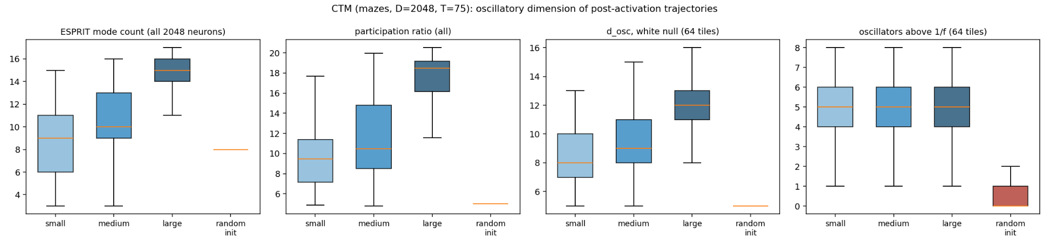
An untrained CTM runs a few damped modes in a strongly synchronised population, and its trajectory is almost independent of the input. The trained model holds about twice as many modes, every one of them on the unit circle (99–100 % with || 0.95, 1–2 % slightly outside it), in a desynchronised population (Table 1, Figure 2).
The modes have periods of roughly 4–17 ticks (inter-quartile range of pole frequency 0.06–0.24 cycles per tick), shorter than the 25-tick memory of the neuron-level models. This is the first empirical anchor for the claim of Section 2.5 that a CTM learns an oscillatory manifold: training does not inherit the oscillators from the architecture, it builds them.
| CTM: trained (large mazes) | CTM: random initial weights (6 seeds) | |
|---|---|---|
| participation ratio | 18.5 | 4.8–5.1 |
| (white null) | 14 | 6 |
| ESPRIT modes in band | 15 | 8 |
| of which sustained, | 15 | 0–4 |
| median pole modulus | 1.00 | 0.92–0.95 |
| pairwise synchrony, mean | 0.15 | 0.43–0.47 |
| oscillators above (tiles) | 5 | 0–2 |
| top-rhythm excess over (tiles / output neurons) | 2.1 / 4.3 | 0.65–1.23 / 0.85–1.42 |
4.2.2 Across training, and against an LSTM baseline
The parity checkpoints supply the contrast that a single maze checkpoint could not: three training runs, CTMs with 25, 50, 75 and 100 ticks and LSTM baselines with the same numbers of ticks, 21 snapshots per run from initialisation to 200 000 iterations (504 checkpoints in all). Each was run on the same 48 input sequences of length 64; = 1 024 neurons for the CTM and 765 units for the LSTM; = /3 (Table 2, Figure 3).
| training iteration | 0 | 10 k | 20 k | 50 k | 100 k | 200 k |
|---|---|---|---|---|---|---|
| CTM, 75 ticks — accuracy | 0.50 | 0.61 | 0.65 | 0.75 | 0.84 | 0.93 |
| pairwise synchrony | 0.45 | 0.27 | 0.24 | 0.21 | 0.20 | 0.19 |
| oscillators above | 0.5 | 3.0 | 5.3 | 5.7 | 5.3 | 5.3 |
| top-rhythm excess | 0.9 | 5.2 | 6.2 | 5.1 | 4.0 | 3.6 |
| participation ratio | 5.1 | 7.2 | 8.3 | 10.6 | 12.5 | 13.4 |
| sustained modes | 0 | 3.0 | 4.0 | 6.0 | 7.7 | 8.7 |
| LSTM, 75 ticks — accuracy | 0.50 | 0.52 | 0.53 | 0.51 | 0.54 | 0.57 |
| pairwise synchrony | 0.81 | 0.53 | 0.51 | 0.62 | 0.58 | 0.46 |
| oscillators above | 0 | 1.0 | 0 | 0 | 1.3 | 1.3 |
| participation ratio | 2.1 | 2.6 | 2.9 | 3.3 | 3.4 | 3.8 |
| sustained modes | 0 | 0.3 | 0.3 | 0.3 | 0.7 | 0.3 |

Training proceeds in two stages, and all six CTM runs with 75 and 100 ticks show them. Within the first 10–20 thousand iterations the population desynchronises (from 0.40–0.46 to 0.21–0.24), the poles move onto the unit circle, and five to six oscillators appear above the aperiodic background where at initialisation there were none to two; that number then stays at five to six for the rest of training. More slowly, and on the time scale of the accuracy curve, the broadband measures grow: the participation ratio from about 5 to between 7 and 21, the sustained modes to between 6 and 13.
The second stage is not tied to success. Of the three runs with 75 ticks, two solve the task perfectly — one with a participation ratio of 7.4 and six sustained modes, after passing through a maximum of 9.0 and contracting, the other with 20.9 and thirteen — and the run that stalls at 79 % accuracy has 12.0 and seven. With 100 ticks the three runs end at 95, 76 and 100 % accuracy with participation ratios of 15.9, 15.9 and 17.1. The broadband dimension is a property of the trained dynamics that varies from seed to seed; the five or six rhythms above the background and the desynchronisation are the part that training produces every time.
The LSTM baselines do not learn the task within 200 000 iterations (53–58 % accuracy) and have almost no oscillatory structure: participation ratio 2–4, zero to two modes and no rhythm above the background with 25, 50 and 75 ticks, from an initial state that is strongly synchronised and heavily damped (synchrony 0.81–0.84, median || 0.58). The 100-tick LSTM is the exception that qualifies the picture: after about 50 000 iterations it acquires six to seven sustained modes and a participation ratio of 9 while its accuracy stays at 52–55 %.
Sustained oscillation is therefore neither sufficient for solving the task nor exclusive to the synchronisation architecture. What distinguishes the CTM on parity is the early and reproducible appearance of rhythms above the background together with desynchronisation; on mazes, where the LSTM baseline does learn, it oscillates as well (Section 6.5–6.6), and the difference between the architectures lies in the cycle rather than in the presence of rhythms.
4.3 Dimension is computation in progress
The oscillatory dimension [1, 6] turns out to measure the regime that the network is in — the time it has spent working — rather than the difficulty of the input as such; the number of rhythms above the aperiodic background does not change with the load; and in this network dimension and synchrony are one axis.
4.3.1 Two regimes: working and done
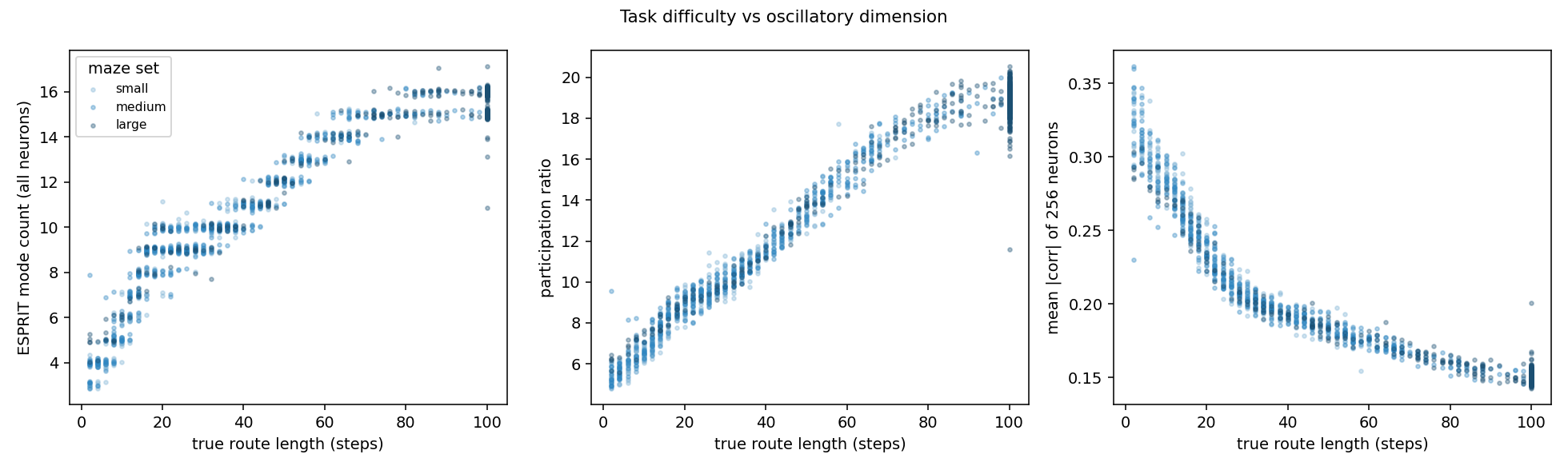
Over the whole trajectory the dimension follows the true route length almost deterministically: Spearman = +0.96 to +0.98 for the mode count, +0.98 to +0.99 for the participation ratio and -0.98 to -0.99 for synchrony in the small and medium sets and in the 200 large mazes whose route is shorter than the 100-step cap; from 3 modes for two-step routes to 16 for routes of 80 steps and more (Table 3, Figure 4).
| steps | set | modes per window | participation ratio | synchrony |
|---|---|---|---|---|
| short, | all sets | 3.0 2.7 2.8 2.9 | 3.5 3.1 3.5 3.4 | 0.41 0.44 0.45 0.44 |
| mid, 15–45 | all sets | 6.7 4.9 3.7 4.4 | 7.4 4.6 3.8 4.9 | 0.31 0.36 0.39 0.37 |
| long, | small | 8.7 8.4 6.4 3.7 | 11.1 9.3 6.0 3.9 | 0.22 0.26 0.32 0.39 |
| long, | large | 8.6 8.9 8.9 8.2 | 11.0 11.4 10.7 9.5 | 0.22 0.22 0.23 0.25 |
While the model is tracing a route it sits in a working regime of about 8.7 modes per window, participation ratio about 11 and synchrony about 0.22, the same in every maze set. When the route is finished it drops into a done regime of about 3 modes, participation ratio 3.5 and synchrony 0.44. The whole-trajectory dimension is therefore the time spent in the working regime, which is why it is proportional to route length; it is a measure of computation still in progress rather than of difficulty as such.
The model’s own certainty falls with route length ( = -0.96 to -0.98) but carries no information about the mode count beyond route length (partial 0), and solved and failed mazes do not differ consistently. The two regimes are the artificial counterpart of the high-dimensional active state and the low-dimensional synchronised state of the BOID framework [1], with the transition set by task completion. The second regime is not final: Section 5.2 shows that it is a rest of fixed length, after which the network returns to work.
4.3.2 Above the aperiodic background the count is invariant
The Monte-Carlo SSA index with the 1/ null finds about five oscillators above the background in every maze set (inter-quartile range 4–6). In the large set this number does not depend on route length ( = -0.02); in the small and medium sets the dependence is weak (+0.57, +0.28). What changes with load is the strength of the dominant rhythm relative to the background, which falls as routes lengthen ( = -0.34 to -0.47). The picture is the one found in cortex: the number of rhythms standing above the background is stable, and the quantity that scales with computational load is the broadband part that energy-rank and white-null estimators count.
4.3.3 Count and synchrony are one axis in the CTM
Across mazes the mode count and pairwise synchrony are strongly anti-correlated ( = -0.94 to -0.97 in the small and medium sets, -0.69 to -0.77 in the large one), and the relation survives removal of route length (partial = -0.12 to -0.33 for the count, -0.46 to -0.69 for the participation ratio).
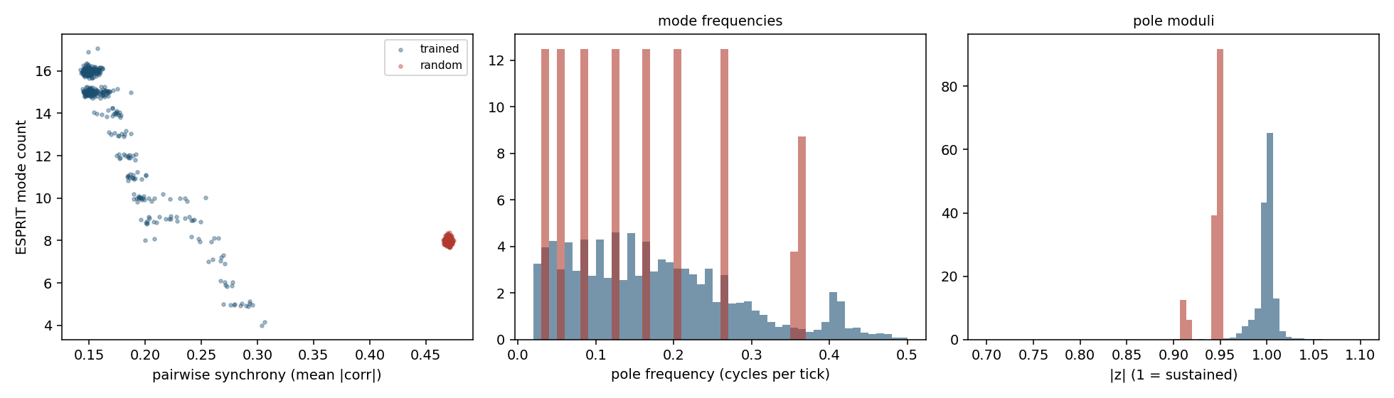
The dissociation between dimension and synchrony observed in cortex is absent here: the pairwise statistic the CTM is trained on and its mode repertoire move together. The expectation stated in Section 3.3 is not supported.
5. Results II: operators, work–rest cycles, and causal modes
5.1 The operator: linear within a regime
Section 2.8 proposed to write the dynamics of a CTM as = + (), with taken from the MSSA decomposition and a learned correction. The decomposition supplies directly [2]: the signal subspace of the block-Hankel matrix defines a shift operator whose eigenvalues are the poles of the modes, and the same subspace forecasts the next sample from the preceding ones [2]; fitted to many trajectories at once, it is the delay-coordinate form of dynamic mode decomposition [34]. The dimension estimates from the BOID framework [1] and from Sections 4.2–4.3 count the modes of this operator. This section measures how much of a trajectory the operator accounts for.
5.1.1 Protocol
The 1 536 trajectories of the three maze sets were pooled and split by input into 960 for fitting, 192 for validation and 384 for testing; every number below is for test inputs. Each neuron was standardised and the population projected on its 64 leading principal axes. These hold 46 % of the variance: the pooled population has a participation ratio of 109 and is not low-dimensional. In this space a linear map from the last ticks to the next one was fitted by ridge regression (the full-rank form of the operator), together with its reduced-rank MSSA form. The score is the share of the tick-to-tick change that is predicted, summed over ticks 25–74. Equation (16) is zero for the prediction that nothing changes and positive when the fitted operator explains part of the state change.
5.1.2 One operator for all inputs
A map from the current state alone predicts 73 % of the change; with eight ticks of history it predicts 86 %, and longer histories add nothing (Figure 7a). Two trivial explanations are excluded. A straight-line extrapolation of the last two states is worse than no change (score -0.93), so the trajectories are not smooth on the scale of a tick. The mean trajectory over the training inputs accounts for 6 % of the variance, so the inputs do not share one trajectory. Started from the true history at tick 25 and then run alone, the operator predicts 76, 73 and 69 % of the change after 5, 10 and 20 ticks (Figure 7b). With 32 or 128 axes in place of 64 the one-step score is 83 and 87%.
5.1.3 What is left for the correction
Adding 4 096 random Fourier features [42] of the same history to the linear map — a kernel approximation of a nonlinear autonomous operator — raises the one-step score from 86 to 89 %. Within the reach of these features the nonlinear part of the autonomous dynamics is small, and the remaining tenth of the change is not a function of the recent state.
5.1.4 Rank
The reduced-rank form needs a rank in the hundreds: with 64 delay modes it is worse than no change, with 256 it predicts 59 %. The pooled dynamics is linear to a good approximation and high-dimensional, in agreement with the participation ratio. At rank 32 the operator has 11 oscillatory poles with || 0.95, and 9 of them recur within 0.02 in two disjoint halves of the training inputs, with periods of 12 to 46 ticks.
5.1.5 Control
The network with random weights is predicted completely by the same construction, for a trivial reason: its trajectory is nearly the same for every input, and the mean trajectory accounts for 97% of its variance. Training moves the network away from one input-independent trajectory, to a state in which a single linear operator still carries most of the dynamics of every input.
Two operators. Ticks were divided by the speed of the state — the mean squared change of the standardised neurons from one tick to the next — with a threshold halfway, on a logarithmic scale, between the level of the shortest routes late in the run and that of the longest routes early in it.
Section 5.2 justifies the division. Fast ticks (work) make up 61 % of the axis and slow ticks (rest) 39 %. An operator fitted on work predicts 88 % of the change on the work ticks of new inputs, and one fitted on rest predicts 95 % on their rest ticks; running alone inside their own regime for 10 ticks they keep 64 % and 89 %. Neither transfers: the work operator applied to rest is far worse than no change, and the rest operator applied to work predicts 13% (Figure 7c). To this approximation the correction of Section 2.8 has a simple form, a switch between two linear operators.
5.1.6 Innovation and dimension
The part of the change that the operator does not predict is a nearly constant fraction of the change itself (Figure 7d): it is large while the state moves and small while it rests. Summed over the run it follows route length ( = +0.92, +0.97 and +0.78 in the small, medium and large sets) and, with it, the measures of Section 4.3.1: participation ratio (+0.91, +0.96, +0.67), mode count (+0.92, +0.96, +0.71) and synchrony (-0.90, -0.95, -0.73). It follows the number of oscillators above the aperiodic background only in the small set (+0.64, against +0.30 and -0.03). This is the division of Section 4.3.2 seen from the side of the operator: the broadband dimension measures activity in progress, and the rhythms above the background belong to the operator.
5.1.7 Operators of single trajectories
Exposinus modes fitted to the first 37 ticks of one trajectory and extrapolated are a weaker predictor than the shared operator. For routes shorter than 15 steps they hold 2 = 0.79 at three ticks and 0.54 at six, where the no-change prediction has 0.72 and -0.05; for routes of 45 steps and more they fail from the first tick (0.03 against 0.55). The operator is a property of the network that is learned across inputs; a single trajectory of 75 ticks does not determine it.
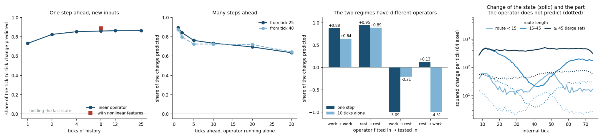
(a) Share of the tick-to-tick change predicted one step ahead by a linear operator shared by all inputs, against the length of the history it uses.
(b) The same operator running alone from the true history.
(c) Operators fitted separately on work and on rest, each tested in both regimes; bars below -1 are cut and labelled.
(d) Squared change of the state per tick and the part of it that the operator does not predict, by route length.
5.2 Work, rest and replay
The regime-switching account of brain states has a high-dimensional active state and a low-dimensional synchronised state of recovery [1]. Section 4.3.1 found their counterparts in the CTM and treated the second as the end of the computation. The speed of the state shows that it is not the end.
5.3 Episodes within the trained horizon
An episode of work is a run of at least three ticks with the speed above the threshold of Section 5.1. Its length is set by the route: the first episode ends at tick 1.1+0.87 route length ( = 0.98; 1 123 mazes of the three sets whose route is below the 100-step cap), which is about one tick per step. The speed then falls by an order of magnitude. After about 31 ticks a second episode begins: in 82–100 % of the mazes with routes of 10 to 45 steps it starts inside the 75 ticks of the training horizon, and for longer routes it is cut off by the end of the axis.
5.3.1 Left running
Nothing in the forward pass depends on the tick index, so the network can be run beyond its horizon. Over 300 ticks (small and medium mazes, 512 of each; threshold set in the same way from the first 75 ticks of each record) the alternation continues, with four to six episodes per maze for routes of 10 to 60 steps (Figure 8a).
The first episode lasts 0.96 and 0.85 ticks per route step in the two sets ( = 0.97 and 0.99). The rest that follows lasts 32 ticks (inter-quartile range 31–33) whatever the route ( = 0.14 and 0.09), and the next rest 33 ticks (31–34) (Figure 8c).
Later episodes are shorter and lose their relation to the route: the second lasts 5 + 0.48 route length in the small set and about 16 ticks in the medium one, the third 12–14 ticks. With the threshold doubled the rest is 36 ticks (34–38). With the threshold halved the rest is split by a small rise of the speed about 15 ticks after the end of work, visible in Figure 8c. In the large set, run for 400 ticks, the first episode follows the route in the same way (0.80 ticks per step, = 0.96) and the first rest lasts 30 ticks for routes of 45 steps and more; after that the alternation is less regular.
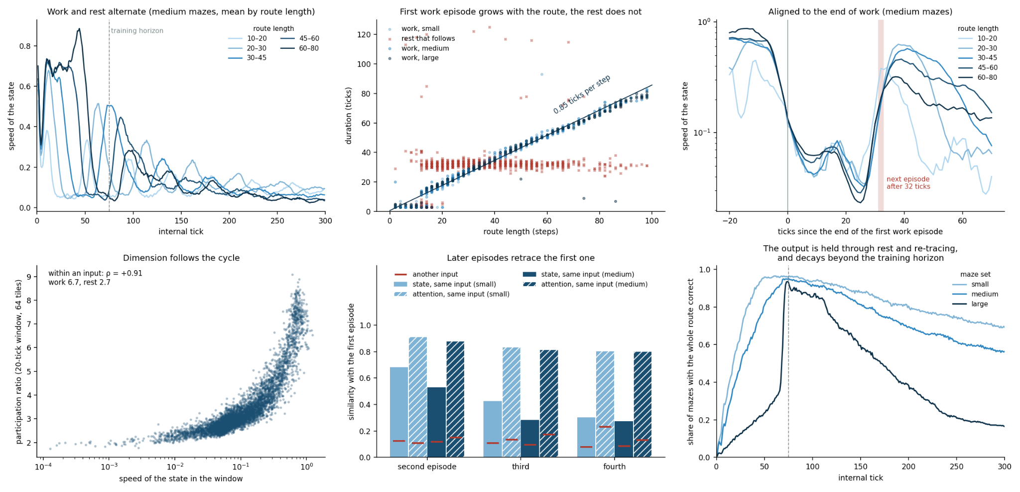
(a) Speed of the state over 300 ticks, mean by route length; the dashed line is the training horizon.
(b) Duration of the first work episode (dots) and of the rest that follows it (crosses) against route length.
(c) Speed aligned to the end of the first work episode; the band is the inter-quartile range of the onset of the next episode.
(d) Participation ratio against the speed of the state in 20-tick windows.
(e) Similarity of later episodes with the first one, for the same maze and for another maze with a route of similar length (red marks).
(f) Share of mazes with the whole route correct.
5.3.2 Replay
A later episode passes through the states of the first one. When the second episode is slid along the first episode of the same maze, the best mean cosine similarity of the states is 0.68 in the small set and 0.53 in the medium set, against 0.12 for the first episode of another maze with a route of similar length; it is higher for the same maze in 97 % and 94 % of the cases. The attention maps agree at 0.91 and 0.88, against 0.11 and 0.15. The best alignment starts 14–17 % into the first episode: the replay skips the initial transient. In the third and fourth episodes the similarity of the states falls to 0.43 and 0.30 (medium set 0.28 and 0.27), while that of the attention maps stays at 0.80–0.84 (Figure 8e). The network looks at the same places again, in the same order.
5.3.3 Output
The route that the model outputs is not disturbed. Its accuracy is 0.97–0.98 during rest and 0.98–0.99 during later episodes, and the share of mazes with the whole route correct — the share of whole routes, the measure of success used below — is 96 % both at tick 50 and at tick 75 in the small set. Beyond the horizon it declines slowly, to 88 % at tick 150 and 69 % at tick 300; in the medium set to 81% and 56 %, and in the large set from 93 % at tick 75 to 60 % and 16 % (Figure 8f).
5.3.4 Dimension
The measures of Section 4.3.1 follow the cycle. In 20-tick windows that lie wholly in work the participation ratio is 6.3–6.8 and pairwise synchrony 0.28–0.30; in windows wholly in rest they are 2.2–2.7 and 0.54–0.60. Within a maze, the speed of the state is correlated with the participation ratio of the window at = +0.90 to +0.93 and with its synchrony at -0.90 to -0.92 (median over mazes; Figure 8d).
The dimension is a property of the regime, and the whole-trajectory dimension of Section 4.3.1 is the share of the axis spent in work, the second episode included.
5.4 What sets the rest
The length of the rest is close to the memory of the neuron-level models, 25 ticks, plus a few ticks; the modes found inside rest have periods of 11–20 ticks, and the small rise of the speed lies half-way through it. The released maze checkpoint has a single memory length, so the relation cannot be tested by comparison on it; Section 5.3 tests it by overwriting the memory, Section 5.6 reads the clock from the weights, and Section 6.1 trains networks with other memory lengths. The parity networks have several memory lengths and do not help: left running for 400 ticks, none of the twelve final checkpoints alternates. Their state settles or drifts, and the accuracy declines. The cycle is something that training on mazes produced, and not a property of the architecture.
5.4.1 Reading
The trained maze CTM is an oscillator on two time scales. On the scale of ticks it is a set of sustained modes governed by a linear operator. On the scale of tens of ticks it alternates between a high-dimensional desynchronised regime, whose duration is the amount of computation, and a low-dimensional synchronised regime of fixed duration, each with its own operator. In the terms of [1], the network does not remain in the active state when the work is done, and it does not remain in the state of recovery either. What the retracing does for the output is tested in Section 5.3.
5.5 What the rest does: holding and restarting
In the brain-state work the low-dimensional state is a state of recovery [1]. What the rest of the CTM is for, and what sets its length, can be asked of the network directly: the forward pass is a loop over ticks whose state can be read and overwritten.
5.5.1 Protocol
The maze CTM was run for 220 ticks on the small and medium sets. A control run gave, for each maze, the tick at which the first work episode ends; the 362 and 410 mazes with 8 105 and a route below the cap were used. Interventions were timed from maze by maze and, unless stated, began at + 5, inside the rest. The measure is the share of mazes whose whole output route is correct.
The second pass is not needed to keep the answer. The synchronisation from which the output is read is accumulated almost without decay: the learned decay is zero for 97 % of the neuron pairs on the output side and for 99.8 % on the attention side. Little can fade, and little needs refreshing. Held in rest — the recurrent state saved at + 5 and restored every 20 ticks, so that the second episode never starts — the network keeps the answer as well as when it is left alone: 98 % and 97 % of the small mazes are correct 30 and 60 ticks after the end of work, against 97 % and 96 %, and in the medium set 96 % and 93 % against 95 % and 90 % (Figure 9a).
With the maze removed (attention output set to zero from + 5) the answer stays at 98–99 % for 100 ticks (medium 93 %), better than when the network is left alone (90 % and 80 %).
The slow loss of the output beyond the training horizon, seen in Section 5.2, therefore comes from the activity that the maze keeps driving, and not from forgetting. The second pass repairs nothing either: the share of correct mazes does not rise during it.
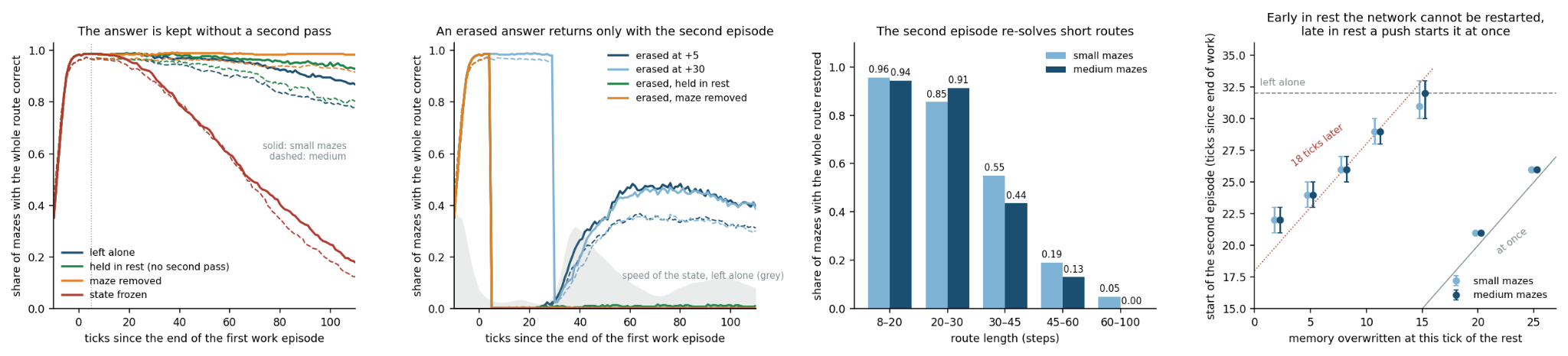
(a) Share of mazes with the whole route correct when the network is left alone, held in rest, deprived of the maze, or frozen.
(b) The same after the accumulated answer is erased 5 or 30 ticks after the end of work, with the network left alone, held in rest, or deprived of the maze; grey: speed of the state when left alone.
(c) Share of mazes whose whole route is restored after erasure at 30 ticks, by route length.
(d) Start of the second episode against the tick of the rest at which the pre-activation memory is overwritten (median and inter-quartile range).
5.5.2 The rest has to move
If the recurrent state is frozen at + 5 instead, the answer is lost: 60 % of the mazes are correct after 60 ticks, and 25 % (medium 18 %) after 100. With accumulation that does not decay, a constant state adds the same products at every tick until they outweigh the answer. The slow oscillation of the resting state (Section 5.2) is what makes rest harmless for the output.
5.5.3 The second episode is a new solution
When the accumulated output is erased at + 5, by re-initialising the output-side synchronisation, the answer does not come back during the rest: 0–3 % of the mazes are correct up to 30 ticks later. It comes back with the second episode, in 58 % of the small mazes within 60 ticks and in 61 % within 100 (medium 42 % and 44 %; Figure 8b). Erasure just before the second episode, at + 30, gives the same shares (59 % and 44 %). If the network is held in rest after the erasure, 2–3% recover; if the maze is removed, 0–1 %. How much is rebuilt depends on the route: 94–96 % of the routes shorter than 20 steps, 85–91 % of those of 20–30 steps, 44–55 % at 30–45 steps, 13–19 % at 45–60 and almost none beyond (Figure 9c). The second episode is shorter than the first (Section 5.2), and it re-solves what fits into it.
5.5.4 The episode starts from inside
With the maze removed the state still leaves rest in every maze, 30 ticks after the end of work (inter-quartile range 29–31, against 32 when left alone); the burst is brief and rebuilds nothing. With the attention output held at its own mean over the rest, 67 % of the small mazes and 90 % of the medium ones start a second episode, at 32 ticks. The timing of the cycle is produced by the recurrent dynamics; the content of an episode needs the maze.
5.5.5 Refractory and excitable rest
The pre-activation memory of every neuron was overwritten with its latest value, as if the current state had lasted for the whole memory. The effect depends on when this is done (Figure 9d). In the first half of the rest the network cannot be restarted: after an overwrite at 2, 5, 8, 11 or 15 ticks the state returns to a quiet that is deeper than before, and the episode begins 20, 19, 18, 18 and 17 ticks after the overwrite. In the second half a push is enough: after an overwrite at 20 or 25 ticks the episode starts on the next tick. The rest is therefore not the time that the memory needs to empty, plus a constant. It has a refractory part of 15–20 ticks, in which a disturbance resets a clock of about 18 ticks, and an excitable part, in which the network fires at the first disturbance and, left alone, fires by itself at 32 ticks. The small rise of the speed half-way through the rest (Section 7.2) lies at the boundary of the two.
5.5.6 Reading
In the maze CTM the low-dimensional regime is a stable store: the answer sits in accumulated synchronisation and survives rest for as long as the resting state keeps oscillating. The return to work is not maintenance. It is the same computation, started again by an excitable recurrent dynamics after a refractory period, and it yields a second and shorter solution of the same maze. The training loss reads two ticks per maze, that of the lowest loss and that of the highest certainty [33], and asks for none of this; the cycle is what the learned dynamics does when it is not being read.
5.6 Modes carry functions, and the clock is a mode
The cycle of Section 5.2 was described by its timing and the rest by its interventions; this section asks which of the modes carry it, and whether the clock of the rest can be read from the weights [2, 1].
5.6.1 Ablation
The operator of Section 5.1 was refitted on the first 75 ticks of 256 control runs on the small set (64 leading axes, the map of the one-tick change) and diagonalised; its eighteen rotating pairs with || 0.9 and periods below 80 ticks have periods of 23, 47, 37, 60, 39, 35, 75 and 60 ticks for the eight strongest (|| 0.955–0.987). At every tick of a run, the modal coordinates of one pair were removed from the postactivations before they enter the synapses and the synchronisation, with the oblique projector -1 that leaves the other modes untouched — two dimensions out of 2 048 — and the network was run for 220 ticks (code/ctm_ablate.py; Figure 10).
The control is a random plane of the same size, removed in the same way. Random planes change nothing: 93–96 % of whole routes correct at tick 75 against 96% when left alone, a rest of 31–33 ticks, a second episode in 73–76 % of the mazes. The modes are not interchangeable. Removing the second mode (period 47) drops the whole routes to 26 %, shortens the rest to 9 ticks (inter-quartile range 4–16) and abolishes the second episode in three mazes out of four (23 % against 75 %): this mode is the clock. Removing the third (period 37) drops the routes to 21 % while the cycle survives — a rest of 38 ticks and a second episode in 78 % — and removing the fourth, fifth and sixth (60, 39, 35) leaves 29–44 % with the cycle intact: these modes carry the answer and not the clock.
The first mode (23 ticks) is almost dispensable (92 %), the seventh and eighth leave 68 %. All rotating modes with || 0.95 removed together leave 13 % and no regimes (speed contrast 2.6 against 24). The two leading principal axes, a non-rotating plane of the same size, leave 29 % and a rest of 6 ticks, since they contain the projections of the slow modes. The rotating modes of the operator are therefore necessary for the computation, one at a time, and the clock of the rest and the content of the answer are different modes.
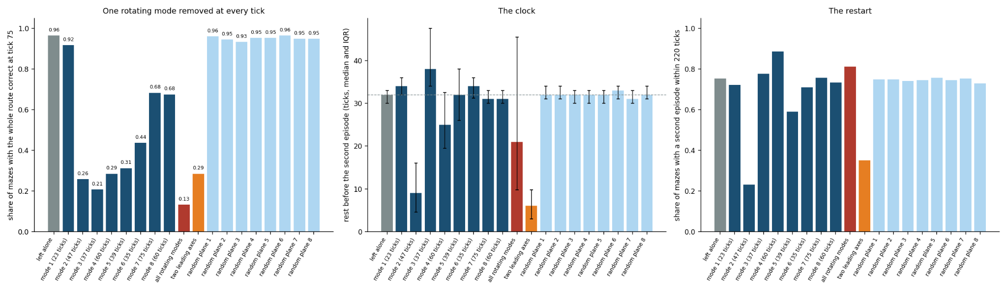
(a) Share of mazes with the whole route correct at tick 75.
(b) Rest before the second episode.
(c) Share of mazes with a second episode within 220 ticks.
5.6.2 Gating
Whether the attention moves in step with the rhythms was tested on the first work episode of 180 mazes with routes long enough for a spectrum: the change of the attention map from one tick to the next against the phase of the dominant rhythm of the state (band-passed around the period of the strongest sustained pole, 5 ticks in the median, and around a fixed 8–14-tick band), with the ticks of the largest changes as events (code/ctm_rhythm_attention.py). The phase-locking value of the attention jumps is 0.20 against a surrogate 95th percentile of 0.43 for the dominant rhythm and 0.25 against 0.42 for the 8–14-tick band, above the surrogate in 9 % and 10 % of the mazes: the rhythms do not set the schedule of the attention.
5.6.3 Coupling
Over 300 ticks, the amplitude of the fast rhythms (periods 6–16 ticks) follows the phase of the slow band (periods 30–100 ticks): a modulation index of 0.035 against a surrogate 95th percentile of 0.031, above it in 66 % of the mazes. This is the alternation of work and rest seen as phase–amplitude coupling — the fast rhythms are large in work and small in rest — and not a mechanism of its own.
5.6.4 The spectrum of the tick map
The map of one tick was linearised from the weights at states of the rest and of the work, for four mazes with routes of 22–42 steps: the state is the pre-activation memory of every neuron (2 048 25 numbers), with the synchronisation accumulators held at their values and the maze fixed, and the 64 eigenvalues of largest modulus of the 51 200 51 200 Jacobian were obtained by Arnoldi iteration with forward-mode automatic differentiation (code/ctm_jacobian.py; about a minute per state). The bulk of the leading spectrum is a band of damped rotating modes with || 0.90–0.95 and periods of 3 to 60 ticks, the repertoire that ESPRIT finds on the trajectories. Two pairs stand out, and they behave the same way in all four mazes. A fast pair with a period of 3 ticks is unstable in the early rest (|| 1.05–1.26 at 3 and 10 ticks after the end of work) and stable by the 24th tick (0.91–0.98): the slow oscillation of the resting state is held up by a fast local instability, and the deepest quiet of the rest, 24 ticks in, is where every mode is damped.
A slow pair with a period of 47–48 ticks is stable at 3 and 10 ticks into the rest (|| 0.94–0.95, periods 52–92), crosses the unit circle 16 to 18 ticks in (|| 1.01–1.04, period 42–50; at the 17th tick 1.02–1.03 with a period of 47–48 in all four mazes; a finer scan of two mazes puts the crossing at the 16th tick and the return below the circle at the 20th), and is below it again at 24 ticks (0.91–0.93). Its period is the period of the clock mode of the ablation, 47 ticks. The two clocks of Section 5.3 follow: a disturbance in the first half of the rest refills the memory and resets the state to the early rest, from which the slow mode takes 17–20 ticks to become unstable again — the 18-tick refractory clock — and a quarter turn of a 47-tick mode after the crossing, about 12 ticks, brings the restart at 30–32 ticks. The rest is a slow rotation that the memory makes unstable at a fixed delay after it is filled; the delay is set by the memory length and the neuron-level models, which is where enters (Section 6.1).
5.6.5 Stopping by the state
The end of the first episode is an internal signal, and Section 5.3 showed that the answer is complete at that point. Stopping the released network two ticks after the speed of the state falls below the threshold gives 98.6 % of whole routes correct on the small set and 96.8 % on the medium set, against 97.8 % and 96.6 % at the fixed horizon of 75 ticks, using 35 and 42 ticks on average — 54 % and 44 % fewer — and 19 ticks for routes under 20 steps against 54–57 for routes over 50. A fixed budget of 50 ticks keeps 97 % on the small set but loses the medium set (82 %). The cost of the computation can follow the route because the network signals its own completion. The attention, recomputed at every tick, is not needed at every tick either: with the attention output recomputed every second tick and held in between, again without retraining, the released network keeps 96.5 % of whole routes on the small set and 95.3 % on the medium set (against 96.5 % and 95.7 %), with the cycle unchanged (rest 32 ticks); every third tick keeps 94.1 % and 92.6 %, every fifth loses the task (59 % and 44 %), and at every eighth the dynamics itself changes (rest of 4 ticks). Half of the attention calls can be dropped at no cost, in agreement with the gating test: the attention is not driven tick by tick by the rhythms (code/ctm_sparse_attention.py).
6. Results III: what sets the regime pattern
Three sets of networks trained here with one recipe separate what belongs to the task from what belongs to the construction [2, 1]: the memory of the neuron-level models is varied, the synchronisation architecture is replaced by an LSTM, and the recurrent core is replaced by the operator of Section 2.8.
6.1 Memory length
Three maze CTMs were trained with the repository’s recipe for small mazes ( = 1 024, = 75, routes capped at 50 steps, 100 000 iterations of batch 64 on one GPU; code/run_queue_M.sh), differing only in the memory length of the neuron-level models: 10, 25 — the value of the released model — and 50.
Snapshots every 5 000 iterations were run for 300 ticks on 256 test mazes, and the final networks on 512, with the measures of Sections 5.2–5.3 (code/train_snap.py, code/ctm_trained_long.py; Figure 10).

(a) Share of test mazes with the whole route correct at tick 75 along training.
(b) The rest before the second episode along training (median and inter-quartile range) for the networks in which fast and slow ticks separate; the dashed line is the released network; the = 25 network restarts in too few mazes for a stable value.
(c) The rest of the final networks against the memory length; the open marker is a network without a division into fast and slow ticks, whose value is not a rest, and the = 25 value rests on the 7 % of mazes that restart.
(d) Median speed of the state aligned to the end of the first work episode, final networks and the released one.
(e) Oscillators above the aperiodic background (solid) and sustained ESPRIT modes (dashed) per trajectory along training, 64 mazes and 75 ticks per snapshot.
6.2 Training
After 100 000 iterations the networks reach a step accuracy of 0.90–0.98 and 37–44 % of whole routes correct at tick 75, against 96 % for the released network after a million iterations on large mazes. They are not trained to convergence; the comparison is between networks at the same stage of one recipe.
= 10. The division into fast and slow ticks is present from 25 000 iterations on (speed contrast 10–17 at every later snapshot, 11 in the final network, against 26 for the released one). The first episode lasts 12.7 + 2.5 route length ticks ( = 0.68, = 0.86), three times slower per step than the released network; the rest that follows lasts 6 ticks (inter-quartile range 4–12), the second episode 7 ticks, and a second episode occurs within 300 ticks in 28 % of the mazes. It replays the first (state cosine 0.80 against 0.20 for another maze, attention 0.99), but from its last quarter — the best alignment starts at 76 % of the first episode — and not from its start. The answer is kept: 41 % of whole routes correct at tick 75, 36 % at tick 300.
= 25. The reference of the recipe, the memory length of the released network, learns least steadily: twice along training, near 25 000 and 55 000 iterations, its state falls almost still (speed contrast 477 and 56, no mode above the background, synchrony 0.47–0.58) and the whole routes drop to 3–9 %, and twice it recovers; it ends at 30 % of whole routes. The final network has the regimes (contrast 27 over 300 ticks; quiet 0.002), the first episode grows with the route (32 + 2.7 route length, = 0.78), and the answer is held through the quiet (step accuracy 0.93 in rest, 30 % of whole routes at tick 75 and 25% at 300) — but it hardly ever restarts: a second episode within 300 ticks in 7 % of the mazes, after 22 ticks (inter-quartile range 10–80). Its quiet is close to a fixed point, like that of the LSTM of Section 6.6, not the slow rotation of the released network. Over the training horizon it carries three sustained modes of period 20 and two above the background, and its operator has six rotating eigenvalues (periods 21 and 29).
= 50. No division into fast and slow ticks at any of the 20 snapshots (contrast 1.0–1.4): the state moves at one speed throughout, the duration of the fast ticks does not follow the route (0.05 ticks per step), later segments do not retrace earlier ones (state cosine 0.10, the level of another maze) although the attention returns to the same places (0.96), and the answer is lost beyond the horizon: 36 % of routes correct at tick 75, 22 % at 150, 10 % at 300.
6.3 Along training
The signature of Section 7.8 on every snapshot (64 mazes, 75 ticks; Figure 10e) shows the rhythms appearing before the task is learned, as on parity (Section 4.2.2). With = 10 the oscillators above the aperiodic background go from 2 to 4 within the first 10 000 iterations, when 18 % of the routes are correct, and their period shortens from 25 to 10 ticks by 40 000; the sustained ESPRIT modes go from 2 to 4 and their period from 24 to 15 ticks; the synchrony in windows falls from 0.53 to 0.44; the contrast of the speed, the measure of the regimes, grows later and more slowly, from 3.5 to 9–11 by 45 000.
With = 50 the count above the background rises from 0 to 3 only by 70 000 iterations, the modes keep a period of 23 ticks throughout, the synchrony stays at 0.54–0.58, and the operator has two to four rotating eigenvalues against eighteen to twenty-six for = 10. The period of the rhythms grows with the memory length, but weakly: 10 ticks at = 10, 11 in the released network at = 25, 13 at = 50.
6.4 Reading
The memory length sets the kind of dynamics that training produces, and the three networks differ in kind rather than in the length of a rest: with = 10 the network separates work from rest, rests for 6 ticks and replays in a quarter of the mazes; with = 25 it separates the regimes, holds its answer in a quiet that is nearly a fixed point, and does not restart; with = 50 it drifts at one speed, keeps no regime and forgets beyond its horizon. The question the experiment was built to answer — whether the 32-tick rest scales with — has no answer at this stage, because only one of the three networks restarts at all: the clock of the released network, a slow mode that the refilled memory destabilises (Section 5.6), is not present in the = 25 network after 100 000 iterations on small mazes, and so it is a product of the longer training, of the larger mazes, or of both, and not of the memory length alone. The direction is nevertheless visible: the shorter the memory, the readier the restart (28 %, 7 %, none), and the longer the memory, the smoother the dynamics; the rhythm’s period grows with only weakly (10, 11, 13 ticks). Closing the comparison needs the three networks trained to convergence.
6.5 A recurrent control: the LSTM
The comparison that the parity baselines could not give — a network that solves the same task without a synchronisation objective — was made on mazes [2, 1]. The repository’s LSTM baseline was trained with the recipe of Section 6.1 (two layers of width 1 024, the same attention over the maze at every tick, the same 75 ticks and certainty-based loss). It reaches 35 % of whole routes at tick 75, the level of the CTMs, and it oscillates: ten sustained ESPRIT modes with a median period of 8 ticks, four oscillators above the aperiodic background at 7 ticks, a participation ratio of 10.6 and a synchrony of 0.24 — more modes than the CTMs trained here (three to four) and than the released one (eight), with five above the background already at 5 000 iterations. Its course is a different pattern. The state moves fast for about 68 ticks whatever the route (60.7 + 0.23 route length, against one tick per step in the released CTM), that is until the training horizon, and then falls almost still (speed 0.002 against 0.24 in work, a contrast of 113; participation ratio 1.9 and synchrony 0.73 in the quiet against 5.3 and 0.35 in work); a second episode occurs within 300 ticks in 30 % of the mazes, after a quiet of 84 ticks with an inter-quartile range of 56–116, and it retraces the first (state cosine 0.42 against 0.22 for another maze, attention 0.94).
Sustained oscillation above the background is therefore not what the synchronisation architecture adds: a recurrent network with attention over a fixed input acquires it on this task as readily, which qualifies the reading of the parity baselines in Section 4.2.2, where the LSTMs that did not oscillate also did not learn.
What the LSTM lacks is the clock: no work in proportion to the route, no rest of fixed length, and a restart that is rare and irregular.
6.6 What its rhythms are
The tests of Sections 5.3 and 5.6 were repeated on it (code/lstm_probe.py). The rhythms belong to the work: eight sustained modes with a period of 8 ticks between ticks 5 and 70, one slow mode in the quiet. They do not need the maze: with the attention output set to zero from tick 30 the speed of the state (0.19 against 0.19) and the modes (5 against 4, three sustained) are unchanged, and the work still ends at tick 66 — the end of work is an internal timer, learned from the horizon, not a reading of the maze. The answer, however, needs the maze: with the input removed the whole routes fall to 2 % within 20 ticks, where the CTM kept 98 %; with the attention held at its mean they stay at 22–25 %. The LSTM has no protected store — its answer is re-read from the input at every tick — and this, not the rhythm, is what the synchronisation accumulators of the CTM add.
The attention moves rhythmically with the state: its tick-to-tick change has autocorrelation peaks at lags 6, 12 and 17, it correlates with the speed of the state ( = 0.36 per tick), and the attention dwells on a cell for 2 ticks (inter-quartile range 1–5), visiting only four cells in 70 ticks — a scan at the period of the rhythm rather than a walk along the route; phase locking of the jumps is at the level of shifted surrogates (0.42 against 0.44), which for a periodic event train is uninformative. The modes are necessary, with a division of labour: the operator fitted to the work has six rotating pairs (periods 42, 30, 20, 6, 50 and 40 ticks, || 0.93–0.97); removing the 6-tick pair ends the work at tick 9 and drops the whole routes from 35 % to 23 % — the fast rhythm is the engine of the work phase — while removing the 30-, 40- or 50-tick pairs leaves the work running to tick 66–68 and drops the routes to 21–24 % — the slow modes carry the content; the 42- and 20-tick pairs are dispensable (32–33 %), all rotating pairs together leave 9 % and no work, and random planes leave 33–34 %.
6.7 A constructed core: the hybrid
The architecture of Section 2.8 — a linear operator as the core and a learned correction — was built into the CTM and trained with the recipe of Section 6.1 at = 10 (code/hybrid.py; three networks on one GPU, 100 000 iterations each). The synapse model of the CTM, a U-Net of 6.2 million parameters that holds 83 % of the network, was replaced by pre = LayerNorm( + in + (, )), where are the post-activations, the attention output, a bank of 512 rotations of 2 2 — one per pair of neurons, each with a learned period, drawn at the start between 4 and 60 ticks, and a learned modulus kept at or below one, which is the exposinus expansion of Section 2.3 written into the weights — and a two-layer correction of width 128. Three cores were trained: the bank with the correction (rot, 1.9 million parameters in all), the bank alone, with the coupling between neurons strictly linear and the only nonlinearity in the neuron-level models (rot_nocorr, 1.6 million), and a dense linear map with the correction and a random start, the control for the rotation structure (lin, 2.9 million). The U-Net network of Section 6.1 (7.5 million) is the reference (Table 4).
| U-Net (CTM) | rotation bank + correction | rotation bank alone | dense linear + correction | |
|---|---|---|---|---|
| parameters | 7.5 M | 1.9 M | 1.6 M | 2.9 M |
| mazes solved at tick 75 | 44 % | 40 % | 37 % | 40 % |
| sustained modes | 4 | 8 | 10 | 5 |
| oscillators above | 3 | 6 | 3 | 4 |
| participation ratio | 6.2 | 11.4 | 9.6 | 8.0 |
| pairwise synchrony | 0.31 | 0.21 | 0.22 | 0.28 |
| speed contrast of the regimes | , no division | |||
| first episode: offset, ticks | 12.7 | 34 | — | 17 |
| first episode: ticks per step | 2.5 (0.86) | 1.1 (0.81) | — | 0.6 (0.60) |
| rest, ticks | 6 [4–12] | 5 [3–26] | — | 15 [6–39] |
| mazes with a restart | 28 % | 69 % | — | 62 % |
| replay, state cosine | 0.80 | 0.38 | 0.22 | |
| forward pass, ms | 62 | 43 | 42 | 42 |
6.8 Accuracy
The three linear cores reach 37–40 % of whole routes against 44 % for the U-Net, with four to five times fewer parameters; the U-Net leads from 25 000 iterations on and the gap at the end is four points. The coupling between neurons can be strictly linear: with the rotation bank alone the computation is carried by the neuron-level models and the attention, at 37 %. The rotation structure is not what buys the accuracy — the dense linear map with a random start does as well — but it is what shapes the dynamics.
6.9 Rhythms
The bank gives the richest repertoire of the list: eight sustained modes and six above the background with a period of 9 ticks, a participation ratio of 11.4 and a synchrony of 0.21, present from 25 000 iterations, against four, three and 6.2 for the U-Net. The periods and moduli of the bank are hardly retuned by training — 14 % of the pairs move their period by more than 20 %, every modulus stays at its starting value of 0.98 — so the network takes the bank as given and learns around it, which says that the particular periods, within 4–60 ticks, matter little.
6.10 Cycle
With the correction, the bank has the regimes of the CTM (contrast 4), a first episode that grows with the route (1.1 ticks per step, = 0.81, from an offset of 34 ticks), a short rest of 5 ticks, a restart in 69 % of the mazes and a replay of the state (0.38 against 0.24 for another maze, attention 0.93). Without the correction the rhythm never stops: ten episodes per maze, no division into fast and slow ticks, and a weak replay (0.22). The dense linear core has regimes and restarts (62 %) but no replay of the state at all (-0.05 against 0.11; the attention does return, 0.95): the rotation structure is what makes the second episode retrace the first.
6.11 Cost
A forward pass of 75 ticks costs 43 ms for the bank against 62 ms for the U-Net at a batch of 64 (0.57 against 0.82 ms per tick): the synapse model was a third of the time of a tick, and the rest — neuron-level models, attention, backbone — is shared by all cores. Mixed precision and a batch of 128 raise the training throughput of the U-Net network from 266 to 422 samples per second on the same GPU; its activations for back-propagation through 75 ticks take 9.9 GB at a batch of 64.
6.12 Reading
The hybrid of Section 2.8 holds on this task: a fixed-structure linear core with a small correction learns the mazes to within four points of the full network at a quarter of the parameters and a third less time per tick, develops the rhythms of the CTM in greater number, and keeps the cycle with its replay when the correction is present. What it does not give is the accuracy of the U-Net at this training budget, and the networks are as far from converged as those of Section 6.1.
7. Other learning systems
The measurement needs three things that the CTM supplies explicitly [2, 1, 6]: an index along which one map is iterated (Section 2.6), channels whose values along the index form the record, and a separation of the network’s own dynamics from the response to its input. The estimators of Section 3.2, the operator of Section 5.1 and the cycle of Sections 5.2–5.3 are architecture-independent. Table 5 summarises the architectures below, ordered by how directly they supply the three.
| architecture | index | channels | iterated map | to separate | first measurement |
|---|---|---|---|---|---|
| CTM [33] | internal tick | post-activations | yes | fixed input | Section 4 |
| RNN, LSTM, GRU; reservoir | position | hidden units | yes; fixed in a reservoir | token stream | poles against local Jacobians (Section 5.1.1); count invariant under training |
| S4, LRU; Mamba | position | state coordinates | linear; selective in Mamba | token stream | count against the poles in the weights |
| UT, ALBERT, DEQ | iteration | residual stream | yes | fixed input | damped or sustained modes; slowing before the halt |
| HRM, TRM | iteration | module states | yes | fixed puzzle | HRM: fixed point, no cycle (measured) |
| language model, generation | generated token | residual stream | closed loop | prompt, noise | no slowing at the answer (measured) |
| diffusion sampler | denoising step | sample coordinates | no (noise level) | none | DDPM: one phase, decided early, PR 1.7 (measured) |
| residual network, depth; neural ODE | layer; solver time | residual stream; state | no (GPT-2, measured); yes | fixed input | per-layer maps only; generator eigenvalues |
| training | optimisation step | weights, loss | approximately | data stream | edge-of-stability modes |
7.1 Recurrence along the sequence
7.1.1 Recurrent networks
An RNN, LSTM or GRU applies one map to its hidden state at every position, +1 = (, ). The hidden units are the channels and the positions the index, so the record is as direct as in a CTM; the difference is that the input changes at every step and drives most of the motion. Two separations are available: the innovation of Section 5.1, which removes what the recent state predicts and leaves the part that the input injects, and the control of Section 5.3, in which the input is held or removed and the network runs on its own. The fixed points and the linearisations around them that are used to read trained recurrent networks [43, 44] are the local version of the Koopman spectrum of Section 2.6. The modes of Section 3.2 are the global one, and they can be compared with the eigenvalues of the local Jacobians. The LSTM baselines of Section 4.2.2 are this case with the input absent after the first ticks.
7.1.2 State-space models
In S4 [45], the linear recurrent unit [44] and their relatives the recurrence is linear with a diagonal complex state matrix, +1 = + , and the output is a linear read-out. The eigenvalues are the poles of Section 2.6, written in the weights; the exposinus expansion is the model’s own parameterisation, not an approximation of it. This makes these models the ground truth for the estimator: the count of Section 3.2 on the hidden states of a trained model should return the poles that the inputs excite, and no others, and the number of poles with || near one that the inputs actually use is the oscillatory dimension of the trained model, available for comparison with the whole set of poles that training left in the weights. In the selective form [46] the step size, and the read-out depend on the input, so the effective operator changes along the sequence; the count then measures the operator that is typical of the sequence, and its variation along the sequence is itself a measurement.
7.1.3 A check with known poles
A diagonal recurrence with eight conjugate pairs (moduli 0.95–1.00, frequencies 0.02–0.30 cycles per step), four inputs and 24 random read-out channels was run under four inputs (code/ssm_ground_truth.py). Running on its own after an impulse, as a CTM runs on a fixed image, the sustained eigenvalues of the operator (|| 0.95; delay coordinates of 10 lags, rank 16–32) return all eight pairs within 0.02 in the -plane and nothing else; the count at the 95 % energy rank returns the five strongest, all correct, and drops the weak damped ones, which is the direction of its bias. Driven by white noise at every step, the energy-rank count is polluted by the drive — eight pairs, of which five are true, with every modulus pushed to one — while the operator at rank 24–32 recovers seven to eight of the eight with at most one spurious pair, and all eight once the input is a regressor of the fit. Driven by narrow-band noise, which excites four of the pairs, both estimators report sustained modes that belong to the drive and not to the network, and regressing the known input out removes only part of them; two pure tones at the frequencies of two poles give exactly those two pairs by either estimator. For a network with a token stream the lesson is the one stated above: the count is exact for the autonomous part of the dynamics, the drive has to be taken out, and a coloured drive is not fully taken out by a linear regressor on the input, so the control of Section 5.3 — the network run with its input held or removed — is the cleaner separation.
7.1.4 A trained state-space model
Two linear recurrent units of 128 complex states each, with a GELU mixing layer after each, were trained on sequential MNIST — 784 pixels, one per step — to 95.9 % in three epochs (code/ssm_trained.py), and the three quantities were compared on 64 test sequences. The weights hold 23 and 16 sustained poles (|| 0.95) in the two layers, out of 128 each; the inputs excite 21 and 26 poles above 1 % of the strongest modal energy, of which 10 and 10 are sustained; and the poles that training placed on the unit circle sit at the harmonics of the input’s structure — periods of 28, 14, 9.3, 4.7 and 4.0 steps, the row of the image and its divisions. Driven by the images, the estimators report that structure and cannot tell the drive from the network: the modes above the background have periods of 4–28 steps and the operator’s rotating eigenvalues periods of 4.0, 4.7, 5.7 and 7.0, all harmonics of 28.
Driven by white noise instead, the same network shows its own repertoire: 14 and 11 sustained poles excited, and the operator’s rotating eigenvalues at periods of 4.0, 9.3, 14.0 and 33.8 steps in the second layer against 4.0, 9.0, 13.6 and 29.4 in its weights, with five oscillators above the background in either case. Three numbers that the framework keeps apart — the repertoire a network has, the part of it an input uses, and the part an estimator sees — are thus all different in a trained model, and the second depends on the input as much as on the network.
7.1.5 Reservoirs
A reservoir computer [47] has a fixed random recurrence and trains only the read-out. Its modes are set by the spectral radius of the recurrence and not by training, which makes it the control that the random-weight CTM of Section 4.2.1 approximates poorly: a network in which the oscillators are built in, so that whatever the read-out learns, the count does not change.
7.2 Iterative inference
Weight-tied depth. Universal transformers (UT) [48] and ALBERT [49] apply one block repeatedly; deep equilibrium models (DEQ) [41] iterate one layer to a fixed point. The iteration is the index, the residual-stream coordinates are the channels, and the input is fixed, so Section 2.6 applies as it stands. A deep equilibrium model is damped by construction — its modes measure the approach to the fixed point and the count is expected to fall to zero as it converges — and a universal transformer with adaptive halting has an internal stop that plays the part of the CTM’s certainty; whether its state slows down before it halts, as the CTM’s does when the route is complete (Section 5.2), is a direct test.
7.2.1 Recursive reasoners
The hierarchical reasoning model [50] couples two recurrent modules, a fast one that iterates for a fixed number of steps and a slow one that is updated once per cycle of the fast one; the tiny recursive model [51] recurses a single network of seven million parameters on its own output for a fixed number of steps. Both solve mazes, Sudoku and ARC puzzles that are out of reach of much larger feed-forward models, and both are the direct analogue of the CTM’s ticks. The questions of Sections 5.2–5.3 are posed to them without change: whether the state moves in episodes, whether there is a rest between them, whether a later episode replays an earlier one, and whether the two time scales that the hierarchical model has by design coincide with the alternation that the CTM learned without being asked.
7.2.2 Measured
The released maze checkpoint of the hierarchical model (27 M parameters; 30 30 mazes with routes of 108–125 steps; two L steps per H step, two H steps per segment, 16 segments at evaluation) was run for 48 segments on 64 test mazes (code/hrm_extract.py, code/hrm_cycles.py).
7.2.3 It contracts
The mean squared change of the L state falls from 1.2 at the first step to 10-4 by the 16th L step and to 10-13 by the 16th segment, by a factor of about 0.68 per L step, the same for solved and unsolved mazes; beyond the horizon nothing moves, and the similarity of later segments with the first ones is 1.000 because the state is constant. The solution is complete after one to four H steps (median two, independent of route length) and never changes afterwards: 77 % of the mazes are solved at the 16th segment and the same 77 % at the 48th, and the unsolved ones settle on a wrong answer at the same rate (token accuracy 0.958 at H steps 8, 32 and 96). The halting head follows the contraction: its margin rises from -7.9 to zero within six H steps and stays there, and the model would halt at H step 2 or 3 in 86 % of the solved mazes. The hierarchical model is thus the case of the deep equilibrium model above — damped modes, a fixed point, no rest and no second episode — and the two time scales of its design produce no alternation. The sustained modes and the cycle of the CTM are not shared by the other recurrent reasoner that solves the same task; they are a property of the CTM’s dynamics, not of recursion on mazes as such.
7.2.4 Diffusion samplers
A diffusion or score-based model [52, 53] generates by iterating a denoising step from noise to data. The trajectory of a sample is the record; the map depends on the noise level, so it is not autonomous, but it changes smoothly along the index, and an operator fitted per noise level is the linearisation of the step there. The early and late steps are known to do different work, coarse structure first and detail last; the expectation is a succession of damped regimes, since the process contracts onto the data manifold, with the dimension measuring how many directions are still being decided at each level. This is the one case in the list where sustained modes would be a defect rather than a finding.
7.2.5 Measured
A pretrained DDPM for 32 32 images (CIFAR-10) was sampled over 200 steps with the deterministic DDIM sampler and with the stochastic DDPM sampler, 256 samples each, recording the sample and the model’s current estimate of the clean image 0() at every step (code/diffusion_extract.py, code/diffusion_cycles.py). The decision is made early and once: with DDIM, 0 correlates 0.5 with the final image at step 41 and 0.9 at step 94, where the signal-to-noise ratio is still 0.07; its speed falls from 0.007 per step to 10-4 by step 40 and to zero afterwards, one fast phase followed by a monotone approach, with no second phase. In 20-step windows the trajectory in the 64 leading axes has a participation ratio of 1.7–1.9 and a synchrony of 0.86–0.89 — a line, not a repertoire — and no pole of a trajectory rotates faster than once per window. A linear map per step predicts 87 % of the step-to-step change early, 55 % in the middle and 7 % late (the mean change alone 56 %, 0 and 0), and a map fitted on one third of the schedule fails on the others, as the map changes with the noise level. With DDPM, the injected noise is the innovation: the decision comes later (0.5 at step 72, 0.9 at step 154), the windows have a participation ratio of 4.3–4.5 and a synchrony of 0.42, and no linear map predicts the step-to-step change (scores at or below zero). The sampler is the contracting case the list expected: damped, decided once, with the dimension of the trajectory set by the injected noise and not by the network.
7.2.6 Energy-based and Hopfield networks
Langevin or asynchronous update iterations on an energy [54] converge to attractors; with symmetric couplings the modes are damped, and with asymmetric couplings limit cycles are possible. The count distinguishes the two.
7.2.7 Generation by a language model
Along the tokens that a language model generates, the residual stream at a fixed layer is a trajectory whose input is the model’s own output: once the prompt is consumed, the loop is closed and the dynamics is autonomous in the sense of Section 2.6, with the sampling noise as the only external term. The division of Section 4.3.1 into work and done has an immediate counterpart in the reasoning and the answer of a chain of thought, and the question of Section 5.2 — whether the state slows down when the answer is reached — can be asked of the residual stream.
7.2.8 Measured
A small instruction-tuned model (Qwen2.5-0.5B-Instruct, 24 layers) solved 64 three-step arithmetic word problems step by step and was made to keep writing after its answer (the end-of-text token suppressed; 220 tokens per problem, the answer line at token 156 in the median, 33 % correct; code/lm_generation.py). The residual stream at layers 6, 12, 18 and 23 was read at every generated token. Nothing slows down when the answer is reached: the speed of the standardised state is 1.1–1.35 per token during the reasoning, 1.0–1.2 on the answer line and 1.05–1.5 afterwards; 20-token windows have the same participation ratio (11–12) and the same synchrony (0.23) before and after the answer.
One operator shared by all problems predicts 55–61 % of the token-to-token change from the current state and 63–67 % with eight tokens of history, and an operator fitted on the reasoning predicts 39–48 % of the change after the answer, against 46–54 % for one fitted there: the segments differ in degree, not in kind. GPT-2 small continuing Wikipedia openings, the control without a task, gives the same picture (speed 1.3–1.6, one-step operator 44–56 %). Along generation, then, the state is driven afresh by every token — consecutive states are only weakly correlated — and the division into work and rest that the CTM shows on a fixed input has no counterpart; what remains to be measured is the part of the change that the token does not explain, with the token embedding as the regressor of Section 5.1, and the same test on a model that reasons well.
7.2.9 A reasoning model
Both were then done on a model that thinks before it answers and re-checks itself as it goes (DeepSeek-R1-Distill-Qwen-1.5B; the same 48 problems, 1 500 tokens each, 75 % correct, the end of the thinking block at token 996 in the median, 6.8 re-checks per problem — “Wait”, “Let me verify”; code/lm_reasoning.py). The trajectory has events but no regimes. At a re-check the speed of the state in the last layer rises by a third (1.23 to 1.61 against 1.27 at random positions) and stays raised for several tokens; at the end of thinking it jumps for one token (0.97 to 1.95) and returns; after the boxed answer the middle layer slows by a quarter (0.74 against 0.95–1.0), the last layer does not.
The dimension and the synchrony in 20-token windows are the same in the thinking and in the answer (10.8 and 0.23 against 10.6 and 0.24), and over 700 tokens the participation ratio is 152 with a synchrony of 0.10, the most extreme stream of the list. The drive is now measured: the token that enters accounts for 17 % (middle layer) to 38 % (last layer) of the token-to-token change on its own, the state for 52–60%, both for 61–79 %; and with the token regressed out the map of the state has no sustained rotating eigenvalue. The part of the residual stream that is its own dynamics contracts; what carries a chain of thought forward from token to token is the text itself and the attention over it.
7.3 Depth as time
7.3.1 Residual networks and transformers
The residual stream of a deep network, +1 = + (), is a dynamical system along depth [55, 56, 57], but with a different map at every layer. The Hankel estimate on this axis describes a trajectory and not an invariant of a map: a mode count along depth is comparable across inputs and across checkpoints of one network, and it is not a count of Koopman modes.
7.3.2 Two things make the axis usable
The middle layers of a trained residual network are to a good approximation interchangeable [57], which is an approximate time-invariance to be tested on the data by the transfer score of Section 5.1, fitting the operator on one range of layers and testing it on the next; and the axis is short, 12 to 100 steps, so the pitfalls of Section 3.4 apply with below a third of the depth and with the rank ceiling reported.
7.3.3 Measured
The residual stream of GPT-2 small (12 blocks, = 768) and medium (24 blocks, = 1 024) was recorded for 128 Wikipedia sequences of 256 tokens, and the share of the layer-to-layer change that a linear map predicts was scored on held-out texts (code/lm_depth.py). A map fitted per layer predicts 94–97 % of the change at the first transition and 80–94 % at the last, but only 35–60 % in the middle layers, where the mean change alone gives 7–20 %.
One map shared by the middle layers predicts 6–40% (small) and 1–48 % (medium). The transfer test fails: the map fitted on the first half of the layers scores 0.02 (small) and -0.13 (medium) on the second half, and the map fitted on the second half -0.09 and -0.17 on the first — no better, or worse, than predicting no change, against 0.23–0.38 on their own layers.
The shared map is close to the identity, with moduli of 0.94–1.11 and rotations whose periods would be 87–99 layers. Depth in these networks is not an iterated map: each layer is its own operator, and a mode count along depth would describe the stack, not a dynamics.
7.3.4 Neural ordinary differential equations
A network defined by a time-invariant vector field [58, 59] is the continuous case of Section 2.6: the Koopman operator of its flow is the object, and the solver’s steps supply the samples. The dimension is then the number of eigenvalues of the generator that the inputs excite, with the real part as damping and the imaginary part as frequency, the continuous form of and .
7.4 Training as time
The weights along optimisation, over the training step , are a multichannel record with the longest axis of all, available from checkpoints at no cost. The oscillations of the loss at the edge of stability [60] are modes of the dynamics of the optimiser on the loss surface, and their count and damping along training are measurable with the instruments of Section 3.2. Section 4.2.2 used the other reading of this axis, the dynamics at each checkpoint; the two readings are complementary, the one measuring how the operator of the network changes, the other what the optimiser does while changing it.
7.5 Two axes at once
A transformer has both depth and position, and its hidden states form a tensor indexed by layer, position and channel. A trajectory matrix in two indices — a block-Hankel embedding along depth nested in one along position — separates modes along the two axes and gives the dimension of each. This is not in the framework of [2] yet; it is the one extension of the method, rather than of its application, that the list requires.
7.6 What has been measured
The order of work followed Table 5. The state-space model came first, as the ground truth against which the estimators are checked (Section 7.1). Of the recursive reasoners, the hierarchical model was run and shows no cycle (Section 7.2); the tiny recursive model has no released weights and remains. The residual stream of a language model was scored along depth (Section 7.3) and along generation, in a small model and in a reasoning one (Section 7.2.7–7.2.9), and a diffusion sampler was run (Section 7.2.4–7.2.5). In every case the first number to report is the share of the one-step change that a shared linear operator predicts, as in Section 5.1: where it is low the modes are not a description of the network, and where it is high the rest of the programme follows.
7.7 Signatures: the pattern of each network
The cycle of Section 5.2 is one pattern; the instruments of Section 3.2 describe the dynamics of any of the networks above in the same terms, and the description is what distinguishes them. For each record of Sections 4–7 — 64 trajectories, a montage of 64 pooled channels, the network’s own axis — the signature is: the participation ratio and the surrogate-thresholded dimension; the ESPRIT modes with their moduli and periods; the oscillators above the 1/ background and their periods; the pairwise synchrony; the dimension and synchrony by thirds of the axis; the speed of the state, its contrast and the number of fast phases; and one linear operator for all trajectories in the 64 leading axes, its one-step share with and without history, and the number of its eigenvalues that are sustained and rotating (code/signature.py, code/make_figs_signature.py; Table 6, Figure 12). The CTM rows are for 64 trajectories of the small maze set on the tile montage, so their counts differ from those of Section 4.2.1, which are for all neurons and the large set.
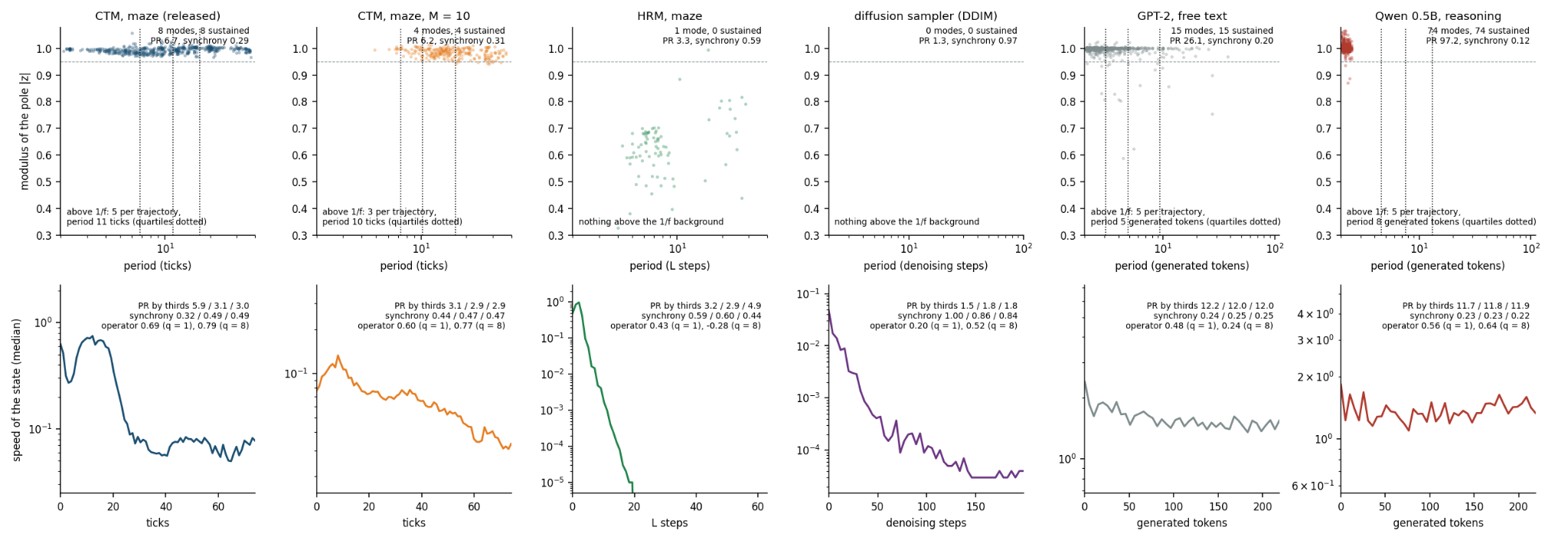
Top: ESPRIT poles of the trajectories, period against modulus, with the quartiles of the periods of the oscillators above the aperiodic background as dotted lines.
Bottom: median speed of the state along the network’s own axis, with the participation ratio and synchrony by thirds and the one-step share of the operator.
| network | PR | modes (sust.) | above : n, period | sync. | PR by thirds | speed contrast; fast phases | operator | rotating |
|---|---|---|---|---|---|---|---|---|
| CTM maze, released, 75 ticks | 6.7 | 8 (8) | 5, 11 ticks | 0.29 | 5.9 / 3.1 / 3.0 | ; 1.7 | 0.69 / 0.79 | 16 (16–23 ticks) |
| the same, 300 ticks | 8.5 | 20 (20) | 6, 20 | 0.28 | 3.3 / 3.0 / 2.8 | ; 4.9 | 0.61 / 0.77 | 26 (20–26) |
| CTM maze, , trained here | 6.2 | 4 (4) | 3, 10 | 0.31 | 3.1 / 2.9 / 2.9 | ; 1.3 | 0.60 / 0.77 | 22 (13–19) |
| CTM maze, | 5.3 | 3 (3) | 2, 7 | 0.35 | 2.7 / 2.9 / 3.2 | ; 1.1 | 0.57 / 0.80 | 6 (21–29) |
| CTM maze, | 5.0 | 3 (3) | 3, 13 | 0.33 | 2.4 / 2.4 / 2.4 | ; 1.6 | 0.56 / 0.80 | 2 (28) |
| LSTM maze, trained here, 75 ticks | 10.6 | 10 (10) | 4, 7 ticks | 0.24 | 5.6 / 5.3 / 4.6 | ; 1.3 | 0.80 / 0.87 | 8 (8–12) |
| LRU, sequential MNIST, 784 steps (trained here) | 17.0 | 15 (15) | 6, 7 steps | 0.32 | — | drive-set | 0.87 / 0.88 | 18 (4–7, harmonics of the row) |
| HRM maze, 64 L steps | 3.3 | 1 (0) | 0 | 0.59 | 3.2 / 2.9 / 4.9 | contraction; 1.0 | 0.43 / | 0 |
| diffusion, DDIM | 1.3 | 0 (0) | 0 | 0.97 | 1.5 / 1.8 / 1.8 | ; 2.3 | 0.20 / 0.52 | 0 |
| diffusion, DDPM | 1.6 | 1 (1) | 1, 8 steps | 0.96 | 2.5 / 3.0 / 4.2 | ; 4.5 | 0.01 / | 0 |
| GPT-2, free text, 220 tokens | 26.1 | 15 (15) | 5, 5 tokens | 0.20 | 12.2 / 12.0 / 12.0 | ; 19.7 | 0.48 / 0.24 | 0 |
| Qwen 0.5B, reasoning, 220 tokens | 97.2 | 74 (74) | 5, 8 tokens | 0.12 | 11.7 / 11.8 / 11.9 | ; 17.2 | 0.56 / 0.64 | 0 |
| R1-distill 1.5B, thinking, 700 tokens | 151.6 | 214 (214) | 4, 13 tokens | 0.10 | 11.3 / 11.0 / 11.0 | ; 46.7 | 0.51 / 0.59 | 0 |
7.7.1 Four patterns appear
The oscillator with regimes (CTM). A repertoire of sustained modes — eight over the training horizon, twenty over 300 ticks, all on the unit circle — of which five or six stand above the aperiodic background, with periods near ten ticks; a dimension that halves from the first third of the axis to the last while the synchrony rises by half, the work and the rest of Section 5.2; a speed with a contrast of 26–30 and, left running, five fast phases in 300 ticks; and an operator that predicts 69 % of the change from the current state, with sixteen to twenty-six rotating eigenvalues of periods 16–26 ticks.
This is a computation carried by rotation, in which the rhythms outlive the task and restart it. The networks trained here (Section 6.1) belong to the same family with fewer rhythms (three), a weaker contrast (9 for = 10) and, at = 50, almost no rotation in the operator (two eigenvalues), the same dimension in every third and a drift at one speed. The LSTM trained on the same mazes is an oscillator too — ten sustained modes, four above the background, an operator that predicts 80 % of the change with eight rotating eigenvalues — and it has regimes (work and a near-still quiet), but its work lasts to the horizon whatever the route and its restart has no clock.
7.7.2 The relaxation (HRM)
One damped mode per trajectory (|| = 0.63, period 7 L steps — the rhythm of the H updates, which come every two L steps and change the input of the L module), nothing above the background, a participation ratio of 3, a synchrony of 0.59, a speed that falls by thirteen orders of magnitude, and an operator with no sustained rotating eigenvalue and a history that does not help (-0.28 with eight steps). The computation is a descent to a fixed point; its only rhythm is the one its schedule imposes.
7.7.3 The line (diffusion)
A participation ratio of 1.3–1.6 and a synchrony of 0.96–0.97: every pixel moves together along one direction, decided in the first fifth of the schedule; no mode, nothing above the background, no rotation. The stochastic sampler adds a noise floor that raises the dimension in the last third (4.2) and lowers the synchrony there (0.47), as the fine detail is written pixel by pixel; its operator predicts nothing, since the change is the noise.
7.7.4 The driven stream (language models along generation)
The highest dimensions of the list — 26 for GPT-2 and 97 for the instruction-tuned model over 220 tokens, 12 in 20-token windows — a synchrony of 0.12–0.20, fifteen to seventy-four sustained poles at periods of two to twenty tokens, and five oscillators above the background at periods of five to eight tokens, the length of a line of text or of one arithmetic step. The speed has no contrast (3) and no slow structure; the dimension is the same in every third of the axis.
The operator predicts half of the change (0.48–0.56) and has not one sustained rotating eigenvalue: the state is rewritten at every token, and the rhythms are those of the text that is written, not of a recurrent dynamics. What persists in these networks persists in the attention cache, which the trajectory of the residual stream does not see.
The count of oscillators above the background is between three and six in every trained network that carries a task along an axis — five or six in the released CTM, two or three in the CTMs trained here, four in the LSTM, six in the state-space model, four or five in the language models — and zero in the relaxation and in the sampler; in the CTM it appears within the first 20 000 iterations of training (Section 4.2.2) and is absent at initialisation. Whether a handful of rhythms above the background is a property of trained networks that carry a task along an axis, or of the estimator at these record lengths, is a question for the networks that remain and for a test on surrogate records of the same length.
7.8 The brain measured the same way
The instruments of Section 7.8 came from recordings of the brain [2, 1], and the comparison can be closed in the other direction: the cortex, taken as one more network and measured with the same montage, the same windows and the same operator. The record is two-photon calcium imaging of mouse cortex — four to ten thousand layer-2/3 neurons at 7.65 Hz with the state of every frame [1] — pooled into the 64 tiles of an 8 8 grid of the field of view and cut into windows of 220 frames (29 s) inside one state: 64 windows each of wake and NREM sleep and 14 of REM from five mice, and 64 of isoflurane anaesthesia with 64 of the wake that precedes it from three (code/brain_records.py) (Table 7).
| state | PR | above : n, period | sync. | PR by thirds | operator | rotating | |
|---|---|---|---|---|---|---|---|
| wake | 62 | 31 | 4, 1.1 s | 0.24 | 10.4 / 10.5 / 9.9 | 0.37 / 0.34 | 0 |
| NREM sleep | 49 | 26 | 3, 2.3 s | 0.24 | 10.5 / 10.3 / 10.7 | 0.30 / 0.27 | 0 |
| REM sleep | 60 | 22 | 3, 5.1 s | 0.13 | 11.7 / 11.3 / 11.5 | 0.26 / 0.04 | 0 |
| wake before anaesthesia | 101 | 24 | 3, 2.1 s | 0.12 | 11.7 / 11.8 / 11.7 | 0.41 / 0.36 | 0 |
| isoflurane anaesthesia | 113 | 34 | 4, 1.6 s | 0.11 | 12.2 / 12.4 / 12.3 | 0.41 / 0.37 | 0 |
By these measures the cortex is a driven stream, the pattern of the language models along generation and not that of the CTM: a participation ratio of 49–62 over a window and 10–12 inside 20-frame windows, a synchrony of 0.11–0.24, three or four oscillators above the aperiodic background with periods of one to five seconds, a state that is rewritten from frame to frame — one shared operator predicts 26–41 % of the change, less than in any of the networks — and no sustained rotating eigenvalue. Inside a window nothing changes: the dimension and the synchrony are the same in every third. The regimes of the brain are on another time scale — minutes — and they separate as the regimes of the CTM do in one respect and not in another.
From wake to NREM sleep the dimension falls (62 to 49; 31 to 26) and the period of the rhythms above the background doubles (1.1 to 2.3 s), the direction of the CTM’s passage from work to rest; but the synchrony does not move (0.24 and 0.24), where in the CTM dimension and synchrony are one axis (Section 4.3.3). The count of oscillators above the background is three to four in every state, the number found in the trained networks that carry a task along an axis (Section 7.8) and absent from the relaxation and the sampler.
Two limits of the comparison are specific to it. The observable is a deconvolved spike estimate at 7.65 Hz, whose fast poles (two frames) are at the edge of the sampling and reflect the estimate as much as the tissue; the rhythms above the background are the part to read. And the cortex is never run on a fixed input: every window is a stream, so the separation of Section 7.1 between the network’s own modes and those of its drive is not available, which is the reason to expect the pattern of a driven stream whatever the cortex’s own repertoire.
8. Dynamical invariants and cognitive functions
The functions named in the opening questions — computing, holding a result, returning to it, keeping time — were built into none of the networks. Each was found as a property of the dynamics that training produced, and each has a formal object [2, 1]; Table 8 collects them. The names are used operationally: a function is what is lost when its object is removed from a running network, or what a network lacks when the object is absent from it.
| function | dynamical object | formal description | shown in |
|---|---|---|---|
| computing | a high-dimensional, desynchronised regime whose duration grows with the size of the problem | regime operator ; high; one step of work per step of the solution | Sections 4.3.1, 5.1, 5.2 |
| holding a result | an integrator outside the oscillating state, and a low-dimensional regime that does not disturb it | accumulators with eigenvalue one; regime operator | Sections 5.5.1–5.5.3 |
| keeping time | a slow rotating mode that crosses the unit circle at a fixed delay after the memory is refilled; a refractory and an excitable phase | an eigenvalue pair of the one-step Jacobian, modulus 1.02–1.04, period 42–50 steps | Sections 5.5.5, 5.6.4 |
| returning to a result | a restart that retraces the first trajectory | rotation in the operator; absent from a dense linear core | Sections 5.3.2, 6.10 |
| knowing that the work is done | the speed of the state falls by an order of magnitude; the network’s own certainty does not track it | a threshold on | Sections 5.3, 5.6.5 |
| looking | attention moves at the period of the fast rhythm in the LSTM, and independently of the rhythms in the CTM | autocorrelation of the change of the attention map; phase locking | Sections 5.6.2, 6.6 |
| learning | the excited eigenvalues move onto the unit circle early; three to six rhythms above the background | along training | Sections 4.2.2, 6.3 |
| a global state | regimes that differ in dimension and, in networks, in synchrony; in cortex, in dimension alone | and pairwise synchrony by state | Sections 4.3, 7.9 |
8.1 What is causal and what is descriptive
Computing, holding, keeping time and returning were each removed or blocked in a running network (Sections 5.3 and 5.6), or are absent from a control that lacks the object (Sections 6.6 and 6.7), and the internal signal of completion was used to stop the network (Section 5.6). The rows on learning and on global states are observations.
8.2 The functions separate
In the model system the content of the answer and the clock are different modes, the store is not the dynamics, and the rhythm is not what distinguishes the network from a control that cannot hold its answer. To say of a trained network that it oscillates is therefore too coarse to be useful; the questions are which modes, in which regime, carrying what.
8.3 The brain
The relation to the brain is of the same kind and has the same limits. The regime-switching account of brain states [1] has a high-dimensional active state and a low-dimensional state of recovery, and replay during rest is its best-known signature. The model system reproduces the alternation, the replay and the dependence of the restart on an internal clock, in a network that was trained only to solve mazes. It does not reproduce the dissociation of dimension from synchrony that the cortex shows (Section 7.9), and the time scales differ by orders of magnitude. The correspondence is between formal objects — a regime, an integrator, a slow mode — and not between mechanisms.
9. Scope and what remains
The results stand on the estimators of [2, 1], on one released maze network, twelve parity networks and seven maze networks trained here far short of convergence; the following limits apply.
Two tasks of the CTM were analysed: mazes — the single released checkpoint and the networks trained here — and parity, with three runs and four tick counts. ImageNet (which needs the validation set), sorting, question answering and reinforcement learning were not. The full work– rest cycle, with its clock, was found in the released maze network only.
Each of the other architectures of Section 7 was measured in one model and one setting — one hierarchical reasoner, two sizes of GPT-2, two small language models, one diffusion sampler, one state-space model, one calcium dataset; the patterns of Section 7.8 describe these cases.
The operator was fitted in the 64 leading axes of the standardised population, which hold less than half of its variance, and the bound on the nonlinear part is that of a kernel approximation with 4096 features; a larger model of the autonomous dynamics could find more.
The division into work and rest depends on a threshold. With the threshold doubled the first episode still grows with the route ( = 0.75) and the rest stays in a narrow range, at 36 ticks (34–38) instead of 32.
Runs beyond 75 ticks are outside the training horizon. The second episode of routes of 10 to 45 steps lies inside it; the later episodes and the slow loss of the output do not.
The spectrum of the tick map (Section 5.6) was computed at six states of four mazes with the synchronisation accumulators held; a scan along the whole rest, and the dependence of the crossing on the memory length, remain. The ablation removes the modal coordinates of a linear fit from a nonlinear network; the random-plane control shows the effect is specific to the modes, not that the modes are the only description of what is removed.
The interventions put the network in states that it has not seen in training (no attention output, a constant memory, an erased output). The variants that stay close to its own states — rest held by restoring a saved state, attention held at its resting mean — lead to the same conclusions where they apply.
The random-weight control for mazes has trajectories that barely depend on the input. The LSTM baselines on parity fail at the task; the LSTM trained on mazes (Section 6.5–6.6) solves it at the level of the CTMs trained here and oscillates, so the rhythms are not specific to the synchronisation architecture, and the comparison that remains open is with a converged LSTM against the released CTM.
The internal time axes are short (25–100 ticks). The slowest resolvable period is about two thirds of the axis, and aperiodic fits rest on a few dozen frequency bins.
The ESPRIT count is not thresholded against a null; the Monte-Carlo SSA index is, and the two answer different questions (Section 4.3.1 against Section 4.3.2).
The broadband dimension is not a marker of task success (Section 4.2.2). What sets its variation between seeds, and how the compact and the expansive solutions of the 75-tick runs differ computationally, are open.
The maze networks trained here (Section 6.1) reach 30–44 % of whole routes against 96 % for the released one; at that stage only the = 10 network restarts, so the dependence of the rest on the memory length is not measured, and the clock of the released network is attributed to its training rather than to by elimination.
Next steps: the hybrid of Section 6.7 with the operator fitted to the released network as its core, so that only the correction is trained; the networks of Sections 6.1 and 6.7 trained to convergence; a bank with periods outside the useful range as the test of whether the periods matter.
10. Conclusion
This paper began from a question that is usually absent from the evaluation of artificial intelligence: what should be measured when a system begins to move from task performance toward strong intelligence? Standard evaluation measures performance from the outside, through benchmarks, outputs, rewards, or accuracy. We have argued that a second object must also be measured: the internal regime organization created by learning.
The starting point was the BOID programme in brain dynamics. There, brain states are not organized by maximal complexity, but by regulated oscillator dimensionality: healthy brains expand dimensionality during conscious engagement and contract it during recovery, sleep, anaesthesia, or efficient trained control, whereas pathological states can reveal failure of dimensional regulation. In the present work, we asked whether trained artificial neural systems can be studied in the same structural language. The answer is not that artificial networks are biological brains. The answer is more precise: some trained artificial systems acquire measurable internal regimes, while others do not.
Using delay embeddings, MSSA, Koopman-mode analysis, BOID-style oscillatory dimensionality, regime-specific operators, and causal mode interventions, we showed that learning can create functional internal dynamics. In the released maze Continuous Thought Machine, training builds sustained oscillatory modes where the untrained architecture has damped ones. The active modes move onto or near the unit circle, a small number of rhythms stand above the aperiodic background, and the computation separates into a high-dimensional desynchronised working regime and a low-dimensional synchronised resting regime. The dimension of the trajectory is therefore not simply a measure of task difficulty; it is a measure of computation still in progress.
The learned dynamics is also structured at the operator level. A single delay-coordinate operator accounts for most of the step-to-step change of the trained maze network, while regime-specific operators describe work and rest separately and fail across the switch. This shows that the nonlinearity of the computation is concentrated, to first approximation, in the transition between regimes. The network is not merely following an uninterpretable high-dimensional flow: it contains identifiable operators, modes, regimes, and switches.
The work–rest cycle is functional. When the network is run beyond its training horizon, it alternates between work and rest, replays its own solution, stores the answer in accumulated synchronisation, and restarts computation through a clock-like mode. The low-dimensional resting regime is not a passive endpoint. It is a stable dynamical state that preserves the output while preparing the system for a new episode. The second episode is not simple persistence of the first answer; it is a partial re-solution of the same maze, triggered by the internal dynamics of the trained system.
These objects are not metaphors. They are causal components of the computation. Removing specific rotating mode pairs selectively disrupts route content or abolishes the restart clock, while removing random planes of the same dimension has little effect. The clock of the rest and the content of the answer are carried by different modes. Conversely, replacing the recurrent core with a bank of rotations plus a small learned correction partially reconstructs the trained dynamics with substantially fewer parameters. Modes, stores, clocks, replay, and regime switching are therefore measurable, predictive, causally testable, and partially buildable components of the learned system.
The broader result is architectural diversity. Measured with the same instruments, different trained systems do not collapse into one dynamical pattern. Some systems form oscillators with regimes; others behave as relaxations, lines, or driven streams. The CTM is not representative of all neural networks, and this is precisely the point. Regime organization is not an automatic consequence of training, scale, or recurrence. It is an emergent structural property of particular learning systems. The difference between architectures is therefore not noise around the result; it is the result.
This conclusion is especially important for the study of strong artificial intelligence. If strong intelligence is defined only by external performance, then increasingly capable systems can only be compared by task score. But if strong intelligence requires internal dimensionality, topology, regime autonomy, self-stabilizing dynamics, stores, clocks, replay, and the capacity to reorganize its own state space, then the internal dynamics of a system becomes an object of experimental measurement. On this view, a system that only maps inputs to outputs remains externally defined, whereas a system that develops functional internal regimes begins to acquire a measurable internal organization.
The implication is also important for small and compact neural systems. The present result is not that a larger model became intelligent. It is almost the opposite: learning can create functional internal dynamics even in compact architectures. This supports a broader view in which structural organization, operator design, functional decomposition, embodied constraints, and regime dynamics may matter more than parameter count alone. Small and lightweight systems are therefore not peripheral to the argument; they show that structurally interesting dynamics can emerge without scaling a model into a giant language model.
We therefore propose that regime switching is one of the first measurable structural markers by which the transition from task-performing artificial systems toward strong artificial intelligence can be studied experimentally. This is not a claim that current networks already possess strong artificial intelligence. It is a proposal for how such a transition can be measured: through the emergence of internal regimes, oscillatory dimensionality, topology, stores, clocks, replay, causal mode structure, and the geometry of possible behaviour spaces.
The contribution of this work is therefore not only an analysis of Continuous Thought Machines. CTM is the first artificial test object in a larger programme. The broader aim is a structural science of intelligence in which natural brains and artificial systems can be compared through measurable properties of their internal dynamics rather than through behavioural analogy alone.
Brain dynamics provided the principle; BOID and MSSA provided the instruments; trained networks provide the artificial systems in which the principle can now be tested. The next step is to determine which architectures can create, stabilize, switch, and reuse internal regimes – and whether regime organization is not only a marker, but a necessary structural condition for strong artificial intelligence.
References
- [1] Bernadotte, A. & Menshikov, I. Brain Oscillator Intrinsic Dimension marks consciousness, recovery mode and failed downshifting in coma. AICumene preprint AiCumene:2026.042v1 (2026). Available at: https://research.aicumene.com/papers/boid-coma/. https://doi.org/10.13140/RG.2.2.31610.25288.
- [2] Bernadotte, A. & Menshikov, I. Multichannel Singular Spectrum Analysis for Estimating Oscillatory Sources and Localizing Attenuating Oscillations. AICumene preprint AiCumene:2026.044v1 (2026). Available at: https://research.aicumene.com/papers/MSSA/. https://doi.org/10.13140/RG.2.2.26719.01442.
- [3] Bernadotte, A. Topology-driven classification of time series. Preprint bioRxiv (2026). https://doi.org/10.64898/2026.04.25.720787.
- [4] Menshikov, I., Elfimov, N. & Bernadotte, A. A Lightweight Hankel-Embedded Pipeline for Real-Time EEG Filtering and Classification. In 2026 12th International Conference on Automation, Robotics and Applications (ICARA), 589–593 (2026). https://doi.org/10.1109/ICARA69401.2026.11480292.
- [5] Bernadotte, A. Estimating the Number of Sources in EEG with Hankel Embedding for Brain-Computer Interface. In 2026 12th International Conference on Automation, Robotics and Applications (ICARA), 621–626 (2026). https://doi.org/10.1109/ICARA69401.2026.11480398.
- [6] Bernadotte, A. & Buchstaber, V. Method for evaluating the number of signal sources and application to non-invasive brain-computer interface. Preprint arXiv arXiv:2410.11844 (2024). https://doi.org/10.48550/arXiv.2410.11844.
- [7] Bernadotte, A. Structural modification of the finite state machine to solve the exponential explosion problem. Programmnaya Ingeneria 13, 449–461 (2022). https://doi.org/10.17587/prin.13.449-461.
- [8] Bernadotte, A. Counter-Augmented Deterministic Automata for Real-Time Regular Expression Matching Without State Explosion. In 2026 12th International Conference on Automation, Robotics and Applications (ICARA), Istanbul, Turkiye, 471–475 (2026). https://doi.org/10.1109/ICARA69401.2026.11480280.
- [9] Bernadotte, A. April Theses of NCP. Talk / presentation (2026). Conceptual theses on measurability of intelligence, language and truth; probabilistic truth and its non-multiplicity. Available at: https://research.aicumene.com/papers/NCP/.
- [10] Gromov, V. A. & Kogan, A. S. Spot the bot: Coarse-Grained Partition of Semantic Paths for Bots and Humans. Preprint arXiv arXiv:2402.17392 (2024).
- [11] Gromov, V. A. & Dang, Q. N. Spot the Bot: Distinguishing Human-Written and Bot-Generated Texts Using Clustering and Information Theory Techniques. In Pattern Recognition and Machine Intelligence, PReMI 2023, Lecture Notes in Computer Science, 20–27 (2023). https://doi.org/10.1007/978-3-031-45170-6_3.
- [12] Gromov, V. A. & Dang, Q. N. Semantic and sentiment trajectories of literary masterpieces. Chaos, Solitons & Fractals 175, 113934 (2023). https://doi.org/10.1016/j.chaos.2023.113934.
- [13] Gromov, V. A., Dang, Q. N. & Yerbolova, A. S. A Language and Its Holes: The First-Order Homology of the Large-Scale Geometrical Structure of a Natural Language. Complexity 2025, 9659172 (2025). https://doi.org/10.1155/cplx/9659172.
- [14] Bernadotte, A. VeNet: a lightweight neural network for efficient brain vessel segmentation in endovascular robotic surgery. Scientific Reports (2026). https://doi.org/10.1038/s41598-026-54176-x.
- [15] Bernadotte, A., Elfimov, N. & Menshikov, I. Semi-automatic annotation of brain vessels in magnetic resonance angiography images. Scientific Data 13, 41 (2026). https://doi.org/10.1038/s41597-025-06354-1.
- [16] Bernadotte, A. & Gromov, V. A. What is Strong AI? Intrinsic Structural Criteria for Strong Intelligence Based on Dimensionality and Topology. AICumene preprint AiCumene:2025.043v1 (2025). Available at: https://research.aicumene.com/papers/StrongAI/. https://doi.org/10.13140/RG.2.2.12211.59681.
- [17] Brown, E. N., Lydic, R. & Schiff, N. D. General anesthesia, sleep, and coma. New England Journal of Medicine 363, 2638–2650 (2010). https://doi.org/10.1056/NEJMra0808281.
- [18] Adam, E. et al. Modulatory dynamics mark the transition between anesthetic states of unconsciousness. Proceedings of the National Academy of Sciences 120, e2300058120 (2023). https://doi.org/10.1073/pnas.2300058120.
- [19] Casali, A. G. et al. A theoretically based index of consciousness independent of sensory processing and behavior. Science Translational Medicine 5, 198ra105 (2013). https://doi.org/10.1126/scitranslmed.3006294.
- [20] Massimini, M., Ferrarelli, F., Huber, R., Esser, S. K., Singh, H. & Tononi, G. Breakdown of cortical effective connectivity during sleep. Science 309, 2228–2232 (2005). https://doi.org/10.1126/science.1117256.
- [21] Casarotto, S. et al. Stratification of unresponsive patients by an independently validated index of brain complexity. Annals of Neurology 80, 718–729 (2016). https://doi.org/10.1002/ana.24779.
- [22] Sarasso, S. et al. Consciousness and complexity during unresponsiveness induced by propofol, xenon, and ketamine. Current Biology 25, 3099–3105 (2015). https://doi.org/10.1016/j.cub.2015.10.014.
- [23] Schartner, M. M. et al. Complexity of multi-dimensional spontaneous EEG decreases during propofol induced general anaesthesia. PLoS ONE 10, e0133532 (2015). https://doi.org/10.1371/journal.pone.0133532.
- [24] Alkire, M. T., Hudetz, A. G. & Tononi, G. Consciousness and anesthesia. Science 322, 876–880 (2008). https://doi.org/10.1126/science.1149213.
- [25] Laureys, S., Owen, A. M. & Schiff, N. D. Brain function in coma, vegetative state, and related disorders. The Lancet Neurology 3, 537–546 (2004). https://doi.org/10.1016/S1474-4422(04)00852-X.
- [26] Roy, R. & Kailath, T. ESPRIT — estimation of signal parameters via rotational invariance techniques. IEEE Transactions on Acoustics, Speech, and Signal Processing 37, 984–995 (1989).
- [27] Golyandina, N., Nekrutkin, V. & Zhigljavsky, A. Analysis of Time Series Structure: SSA and Related Techniques. Chapman & Hall/CRC (2001).
- [28] Takens, F. Detecting strange attractors in turbulence. In Dynamical Systems and Turbulence, Warwick 1980, Lecture Notes in Mathematics 898, 366–381 (1981).
- [29] Broomhead, D. S. & King, G. P. Extracting qualitative dynamics from experimental data. Physica D 20, 217–236 (1986).
- [30] Menshikov, I., Orlov, K., Berestov, V. & Bernadotte, A. Preoperative personalized vascular 3D simulator of the intelligent robotic ecosystem LevshaAI for endovascular neurosurgery. In 2023 9th International Conference on Automation, Robotics and Applications (ICARA), 6–10 (2023). https://doi.org/10.1109/ICARA56516.2023.10125981.
- [31] Menshikov, I. & Bernadotte, A. Intelligent robotic motion copying system LevshaAI for neurosurgical endovascular operations with haptic feedback and preoperative personalized simulation. In 2022 IEEE International Conference on Cyborg and Bionic Systems (CBS), 386–391 (2023). https://doi.org/10.1109/CBS55922.2023.10115398.
- [32] Bernadotte, A. Cyber security for surgical remote intelligent robotic systems. In 2023 9th International Conference on Automation, Robotics and Applications (ICARA), 65–69 (2023). https://doi.org/10.1109/ICARA56516.2023.10126050.
- [33] Darlow, L., Regan, C., Risi, S., Seely, J. & Jones, L. Continuous Thought Machines. Preprint arXiv arXiv:2505.05522 (2025). Available at: https://github.com/SakanaAI/continuous-thought-machines.
- [34] Schmid, P. J. Dynamic mode decomposition of numerical and experimental data. Journal of Fluid Mechanics 656, 5–28 (2010).
- [35] Koopman, B. O. Hamiltonian systems and transformation in Hilbert space. Proceedings of the National Academy of Sciences USA 17, 315–318 (1931).
- [36] Mezić, I. Spectral properties of dynamical systems, model reduction and decompositions. Nonlinear Dynamics 41, 309–325 (2005).
- [37] Rowley, C. W., Mezić, I., Bagheri, S., Schlatter, P. & Henningson, D. S. Spectral analysis of nonlinear flows. Journal of Fluid Mechanics 641, 115–127 (2009).
- [38] Williams, M. O., Kevrekidis, I. G. & Rowley, C. W. A data-driven approximation of the Koopman operator: extending dynamic mode decomposition. Journal of Nonlinear Science 25, 1307–1346 (2015).
- [39] Arbabi, H. & Mezić, I. Ergodic theory, dynamic mode decomposition, and computation of spectral properties of the Koopman operator. SIAM Journal on Applied Dynamical Systems 16, 2096–2126 (2017).
- [40] Sauer, T., Yorke, J. A. & Casdagli, M. Embedology. Journal of Statistical Physics 65, 579–616 (1991). https://doi.org/10.1007/BF01053745.
- [41] Allen, M. R. & Smith, L. A. Monte Carlo SSA: detecting irregular oscillations in the presence of colored noise. Journal of Climate 9, 3373–3404 (1996).
- [42] Rahimi, A. & Recht, B. Random features for large-scale kernel machines. In Advances in Neural Information Processing Systems 20 (2007).
- [43] Sussillo, D. & Barak, O. Opening the black box: low-dimensional dynamics in high-dimensional recurrent neural networks. Neural Computation 25, 626–649 (2013).
- [44] Orvieto, A. et al. Resurrecting recurrent neural networks for long sequences. In International Conference on Machine Learning (2023). Preprint arXiv arXiv:2303.06349.
- [45] Gu, A., Goel, K. & Ré, C. Efficiently modeling long sequences with structured state spaces. In International Conference on Learning Representations (2022). Preprint arXiv arXiv:2111.00396.
- [46] Gu, A. & Dao, T. Mamba: linear-time sequence modeling with selective state spaces. Preprint arXiv arXiv:2312.00752 (2023).
- [47] Jaeger, H. & Haas, H. Harnessing nonlinearity: predicting chaotic systems and saving energy in wireless communication. Science 304, 78–80 (2004).
- [48] Dehghani, M., Gouws, S., Vinyals, O., Uszkoreit, J. & Kaiser, L. Universal Transformers. In International Conference on Learning Representations (2019). Preprint arXiv arXiv:1807.03819.
- [49] Lan, Z., Chen, M., Goodman, S., Gimpel, K., Sharma, P. & Soricut, R. ALBERT: a lite BERT for self-supervised learning of language representations. In International Conference on Learning Representations (2020). Preprint arXiv arXiv:1909.11942.
- [50] Wang, G. et al. Hierarchical Reasoning Model. Preprint arXiv arXiv:2506.21734 (2025).
- [51] Jolicoeur-Martineau, A. Less is More: Recursive Reasoning with Tiny Networks. Preprint arXiv arXiv:2510.04871 (2025).
- [52] Ho, J., Jain, A. & Abbeel, P. Denoising diffusion probabilistic models. In Advances in Neural Information Processing Systems 33 (2020).
- [53] Song, Y., Sohl-Dickstein, J., Kingma, D. P., Kumar, A., Ermon, S. & Poole, B. Score-based generative modeling through stochastic differential equations. In International Conference on Learning Representations (2021). Preprint arXiv arXiv:2011.13456.
- [54] Hopfield, J. J. Neural networks and physical systems with emergent collective computational abilities. Proceedings of the National Academy of Sciences USA 79, 2554–2558 (1982).
- [55] Haber, E. & Ruthotto, L. Stable architectures for deep neural networks. Inverse Problems 34, 014004 (2018).
- [56] E, W. A proposal on machine learning via dynamical systems. Communications in Mathematics and Statistics 5, 1–11 (2017).
- [57] Veit, A., Wilber, M. & Belongie, S. Residual networks behave like ensembles of relatively shallow networks. In Advances in Neural Information Processing Systems 29 (2016).
- [58] Chen, R. T. Q., Rubanova, Y., Bettencourt, J. & Duvenaud, D. Neural ordinary differential equations. In Advances in Neural Information Processing Systems 31 (2018).
- [59] Rubanova, Y., Chen, R. T. Q. & Duvenaud, D. Latent ODEs for irregularly-sampled time series. In Advances in Neural Information Processing Systems 32 (2019).
- [60] Cohen, J. M., Kaur, S., Li, Y., Kolter, J. Z. & Talwalkar, A. Gradient descent on neural networks typically occurs at the edge of stability. In International Conference on Learning Representations (2021). Preprint arXiv arXiv:2103.00065.
- [61] Gromov, M. Great Circle of Mysteries: Mathematics, the World, the Mind. Birkhäuser/Springer (2018). https://doi.org/10.1007/978-3-319-53049-9.
- [62] Buchstaber, V. M. Time series analysis and Grassmannians. In Applied Problems of Radon Transform, American Mathematical Society Translations, Series 2, 162, 1–17 (1994).
- [63] Kuramoto, Y. Chemical Oscillations, Waves, and Turbulence. Springer (1984).
- [64] Brunton, S. L., Brunton, B. W., Proctor, J. L., Kaiser, E. & Kutz, J. N. Chaos as an intermittently forced linear system. Nature Communications 8, 19 (2017).
- [65] Bai, S., Kolter, J. Z. & Koltun, V. Deep equilibrium models. In Advances in Neural Information Processing Systems 32 (2019).
- [66] Elhage, N., Nanda, N., Olsson, C. et al. A mathematical framework for transformer circuits. Transformer Circuits Thread (2021). Available at: https://transformer-circuits.pub/2021/framework/.
- [67] Maheswaranathan, N., Williams, A. H., Golub, M. D., Ganguli, S. & Sussillo, D. Universality and individuality in neural dynamics across large populations of recurrent networks. In Advances in Neural Information Processing Systems 32 (2019).
- [68] Gosseries, O., Di, H., Laureys, S. & Boly, M. Measuring consciousness in severely damaged brains. Annual Review of Neuroscience 37, 457–478 (2014). https://doi.org/10.1146/annurev-neuro-062012-170339.
- [69] Deco, G. & Jirsa, V. K. Ongoing cortical activity at rest: criticality, multistability, and ghost attractors. Journal of Neuroscience 32, 3366–3375 (2012). https://doi.org/10.1523/JNEUROSCI.2523-11.2012.
- [70] Breakspear, M. Dynamic models of large-scale brain activity. Nature Neuroscience 20, 340–352 (2017). https://doi.org/10.1038/nn.4497.
- [71] Kelso, J. A. S. Multistability and metastability: understanding dynamic coordination in the brain. Philosophical Transactions of the Royal Society B 367, 906–918 (2012). https://doi.org/10.1098/rstb.2011.0351.
- [72] Tognoli, E. & Kelso, J. A. S. The metastable brain. Neuron 81, 35–48 (2014). https://doi.org/10.1016/j.neuron.2013.12.022.
- [73] Friston, K. The free-energy principle: a unified brain theory? Nature Reviews Neuroscience 11, 127–138 (2010). https://doi.org/10.1038/nrn2787.
- [74] Stringer, C., Pachitariu, M., Steinmetz, N., Reddy, C. B., Carandini, M. & Harris, K. D. Spontaneous behaviors drive multidimensional, brain-wide activity. Science 364, eaav7893 (2019). https://doi.org/10.1126/science.aav7893.
- [75] Cunningham, J. P. & Yu, B. M. Dimensionality reduction for large-scale neural recordings. Nature Neuroscience 17, 1500–1509 (2014). https://doi.org/10.1038/nn.3776.
- [76] Gallego, J. A., Perich, M. G., Miller, L. E. & Solla, S. A. Neural manifolds for the control of movement. Neuron 94, 978–984 (2017). https://doi.org/10.1016/j.neuron.2017.05.025.
- [77] Gallego, J. A., Perich, M. G., Chowdhury, R. H., Solla, S. A. & Miller, L. E. Long-term stability of cortical population dynamics underlying consistent behavior. Nature Neuroscience 23, 260–270 (2020). https://doi.org/10.1038/s41593-019-0555-4.
- [78] Vyas, S., Golub, M. D., Sussillo, D. & Shenoy, K. V. Computation through neural population dynamics. Annual Review of Neuroscience 43, 249–275 (2020). https://doi.org/10.1146/annurev-neuro-092619-094115.
- [79] Mante, V., Sussillo, D., Shenoy, K. V. & Newsome, W. T. Context-dependent computation by recurrent dynamics in prefrontal cortex. Nature 503, 78–84 (2013). https://doi.org/10.1038/nature12742.
- [80] Remington, E. D., Narain, D., Hosseini, E. A. & Jazayeri, M. Flexible sensorimotor computations through rapid reconfiguration of cortical dynamics. Neuron 98, 1005–1019.e5 (2018). https://doi.org/10.1016/j.neuron.2018.05.020.
- [81] Sadtler, P. T. et al. Neural constraints on learning. Nature 512, 423–426 (2014). https://doi.org/10.1038/nature13665.
- [82] Churchland, M. M. et al. Neural population dynamics during reaching. Nature 487, 51–56 (2012). https://doi.org/10.1038/nature11129.
- [83] Rabinovich, M. I., Simmons, A. N. & Varona, P. Dynamical bridge between brain and mind. Trends in Cognitive Sciences 19, 453–461 (2015). https://doi.org/10.1016/j.tics.2015.06.005.
- [84] Rabinovich, M. I., Huerta, R., Varona, P. & Afraimovich, V. S. Transient cognitive dynamics, metastability, and decision making. PLoS Computational Biology 4, e1000072 (2008). https://doi.org/10.1371/journal.pcbi.1000072.
- [85] Sompolinsky, H., Crisanti, A. & Sommers, H. J. Chaos in random neural networks. Physical Review Letters 61, 259–262 (1988). https://doi.org/10.1103/PhysRevLett.61.259.
- [86] Maass, W., Natschläger, T. & Markram, H. Real-time computing without stable states: a new framework for neural computation based on perturbations. Neural Computation 14, 2531–2560 (2002). https://doi.org/10.1162/089976602760407955.
- [87] Pascanu, R., Mikolov, T. & Bengio, Y. On the difficulty of training recurrent neural networks. In International Conference on Machine Learning (2013). Preprint arXiv arXiv:1211.5063.
- [88] Hochreiter, S. & Schmidhuber, J. Long short-term memory. Neural Computation 9, 1735–1780 (1997). https://doi.org/10.1162/neco.1997.9.8.1735.
- [89] Graves, A. Adaptive computation time for recurrent neural networks. Preprint arXiv arXiv:1603.08983 (2016).
- [90] Graves, A. et al. Hybrid computing using a neural network with dynamic external memory. Nature 538, 471–476 (2016). https://doi.org/10.1038/nature20101.
- [91] Banino, A. et al. Vector-based navigation using grid-like representations in artificial agents. Nature 557, 429–433 (2018). https://doi.org/10.1038/s41586-018-0102-6.
- [92] Ha, D. & Schmidhuber, J. World models. Preprint arXiv arXiv:1803.10122 (2018).
- [93] Hafner, D., Lillicrap, T., Ba, J. & Norouzi, M. Dream to control: learning behaviors by latent imagination. In International Conference on Learning Representations (2020). Preprint arXiv arXiv:1912.01603.
- [94] Hafner, D., Lillicrap, T., Norouzi, M. & Ba, J. Mastering Atari with discrete world models. In International Conference on Learning Representations (2021). Preprint arXiv arXiv:2010.02193.
- [95] Sutton, R. S. Dyna, an integrated architecture for learning, planning, and reacting. ACM SIGART Bulletin 2, 160–163 (1991). https://doi.org/10.1145/122344.122377.
- [96] Buzsaki, G. Rhythms of the Brain. Oxford University Press (2006).
- [97] Buzsaki, G. The Brain from Inside Out. Oxford University Press (2019).
- [98] Foster, D. J. Replay comes of age. Annual Review of Neuroscience 40, 581–602 (2017). https://doi.org/10.1146/annurev-neuro-072116-031538.
- [99] Wilson, M. A. & McNaughton, B. L. Reactivation of hippocampal ensemble memories during sleep. Science 265, 676–679 (1994). https://doi.org/10.1126/science.8036517.
- [100] Peyrache, A., Khamassi, M., Benchenane, K., Wiener, S. I. & Battaglia, F. P. Replay of rule-learning related neural patterns in the prefrontal cortex during sleep. Nature Neuroscience 12, 919–926 (2009). https://doi.org/10.1038/nn.2337.
- [101] Perea, J. A. & Harer, J. Sliding windows and persistence: an application of topological methods to signal analysis. Foundations of Computational Mathematics 15, 799–838 (2015). https://doi.org/10.1007/s10208-014-9206-z.
- [102] Edelsbrunner, H., Letscher, D. & Zomorodian, A. Topological persistence and simplification. Discrete & Computational Geometry 28, 511–533 (2002). https://doi.org/10.1007/s00454-002-2885-2.
- [103] Ghrist, R. Barcodes: the persistent topology of data. Bulletin of the American Mathematical Society 45, 61–75 (2008). https://doi.org/10.1090/S0273-0979-07-01191-3.
- [104] Packard, N. H., Crutchfield, J. P., Farmer, J. D. & Shaw, R. S. Geometry from a time series. Physical Review Letters 45, 712–716 (1980). https://doi.org/10.1103/PhysRevLett.45.712.
- [105] Kennel, M. B., Brown, R. & Abarbanel, H. D. I. Determining embedding dimension for phase-space reconstruction using a geometrical construction. Physical Review A 45, 3403–3411 (1992). https://doi.org/10.1103/PhysRevA.45.3403.
- [106] Grassberger, P. & Procaccia, I. Characterization of strange attractors. Physical Review Letters 50, 346–349 (1983). https://doi.org/10.1103/PhysRevLett.50.346.
- [107] Turing, A. M. Computing machinery and intelligence. Mind 59, 433–460 (1950). https://doi.org/10.1093/mind/LIX.236.433.
- [108] Newell, A. & Simon, H. A. Computer science as empirical inquiry: symbols and search. Communications of the ACM 19, 113–126 (1976). https://doi.org/10.1145/360018.360022.
- [109] Legg, S. & Hutter, M. Universal intelligence: a definition of machine intelligence. Minds and Machines 17, 391–444 (2007). https://doi.org/10.1007/s11023-007-9079-x.
- [110] Chollet, F. On the measure of intelligence. Preprint arXiv arXiv:1911.01547 (2019).
- [111] Lake, B. M., Ullman, T. D., Tenenbaum, J. B. & Gershman, S. J. Building machines that learn and think like people. Behavioral and Brain Sciences 40, e253 (2017). https://doi.org/10.1017/S0140525X16001837.
- [112] LeCun, Y. A path towards autonomous machine intelligence. OpenReview preprint (2022).
- [113] Bengio, Y. The consciousness prior. Preprint arXiv arXiv:1709.08568 (2017).
- [114] Dehaene, S., Kerszberg, M. & Changeux, J.-P. A neuronal model of a global workspace in effortful cognitive tasks. Proceedings of the National Academy of Sciences USA 95, 14529–14534 (1998). https://doi.org/10.1073/pnas.95.24.14529.
- [115] Dehaene, S. & Changeux, J.-P. Experimental and theoretical approaches to conscious processing. Neuron 70, 200–227 (2011). https://doi.org/10.1016/j.neuron.2011.03.018.